Frequentist Evaluation — Paired Laplace

This page is the paired counterpart of Frequentist Evaluation: it answers the same four diagnostic questions but for the paired procedure built around the Laplace-approximation model PairedBayesPropTest and its sequential variant SequentialPairedBayesPropTest.

The data contract is paired binary outcomes — every observation \(i \in \{1,\dots,n\}\) contributes a pair \((y_{A,i}, y_{B,i})\). The analysis model is

\[ y_{A,i} \sim \text{Bern}\bigl(\sigma(\mu + \delta_A)\bigr), \qquad y_{B,i} \sim \text{Bern}\bigl(\sigma(\mu)\bigr), \]

with prior \(\delta_A \sim \mathcal{N}(0, \sigma_\delta^2)\) on the logit-scale effect. The Savage–Dickey BF tests \(H_0: \delta_A = 0\), equivalent to \(H_0: p_A = p_B\).

For the complementary sample-size planning question see BFDA. For the underlying decision-rule conventions see Decision Rules.

What to estimate

Diagnostic	What it answers
Three-way OC	P(reject H₀), P(accept H₀), P(inconclusive) as functions of the true effect Δ = p_A − p_B
Null-decision sweep	P(reject H₀ \| Δ = 0) swept over the baseline rate p_B (the logit prior on δ_A is not translation-invariant on the probability scale)
CI coverage	Frequentist coverage of the 95 % credible interval on Δ derived from the Laplace posterior
Sequential stopping-time distribution	Empirical distribution of the per-arm sample size at which SequentialPairedBayesPropTest stops

Three-way decision classifier

The same classify_bf helper is used here so the simulated OC analysis and the deployed sequential paired procedure share one decision boundary:

from bayesprop.resources.bayes_nonpaired import classify_bf
from bayesprop.resources.bayes_paired import PairedBayesPropTest

bf10 = PairedBayesPropTest().fit(y_A, y_B).savage_dickey_test().BF_10
category = classify_bf(bf10, bf_upper=3.0, bf_lower=1.0 / 3.0)
# → "reject" | "accept" | "inconclusive"

See Decision Rules → Three-way classification for the threshold conventions.

Frequentist baseline (McNemar's exact test)

For paired binary data the canonical frequentist analogue of Fisher's exact test is McNemar's exact test, which conditions on the discordant pairs \(b = \#\{i: y_{A,i}=1, y_{B,i}=0\}\) and \(c = \#\{i: y_{A,i}=0, y_{B,i}=1\}\). Under \(H_0: p_A = p_B\) and conditional on \(b+c\), \(b \sim \text{Binomial}(b+c, 0.5)\). The library ships a small wrapper that mirrors the data contract of the Bayesian paired test:

from bayesprop.utils.utils import mcnemar_paired_test, simulate_paired_scores

sim = simulate_paired_scores(N=200, theta_A=0.62, theta_B=0.50)
freq = mcnemar_paired_test(sim.y_A, sim.y_B)
print(f"McNemar p = {freq.p_value:.4f},  OR = {freq.odds_ratio}")

The exact binomial p-value is used when the discordant count \(b + c \leq 25\); otherwise the standard \(\chi^2\) approximation is used. As in the non-paired case the most useful application is as a calibration reference: pick a frequentist \(\alpha\) such that the empirical Type-I rate at \(\Delta = 0\) matches the Bayes BF rule's Type-I rate, then overlay the two power curves.

Pre-built OC simulation harness

The full simulation logic — grid sweeps for the three-way OC plot, matched-\(\alpha\) calibration, CI coverage tracking, Wilson Monte-Carlo bands and the sequential stopping-time distribution — lives in bayesprop.utils.operation_characteristics_paired. The notebook src/notebooks/operating_characteristics_paired_laplace.ipynb is a thin orchestration layer on top of it, so you can call the same functions directly from your own scripts:

import numpy as np
from bayesprop.utils.operation_characteristics_paired import (
    grid_fixed_n_paired,
    matched_calibration_alpha,
    simulate_sequential_paired,
    wilson_band,
)

grid = [(round(0.6 + d, 4), 0.6) for d in np.linspace(-0.2, 0.2, 11)]
df_oc, pvals = grid_fixed_n_paired(
    grid, n=200, n_sim=400, seed=20260514,
    prior_sigma_delta=1.0, bf_upper=3.0, bf_lower=1.0 / 3.0,
)
idx_null = int(np.argmin(np.abs(df_oc["delta"])))
alpha_matched = matched_calibration_alpha(
    pvals, df_oc.iloc[idx_null]["reject"], idx_null,
)
lo, hi = wilson_band(df_oc["reject"].to_numpy(), n_sim=400)

seq = simulate_sequential_paired(
    p_A=0.75, p_B=0.55, n_sim=80, rng=np.random.default_rng(0),
    n_min=50, n_max=600, batch_size=50,
)

See API → Operating Characteristics (Paired) for the full reference.

Worked example — the four diagnostic plots

The plots below are produced end-to-end by the paired notebook above with p_B = 0.6, n pairs = 200, M = 400 replicates, prior \(\sigma_\delta = 1.0\) on the logit-scale effect, and BF thresholds \((3, 1/3)\). Shaded bands are 95 % Wilson Monte-Carlo bands.

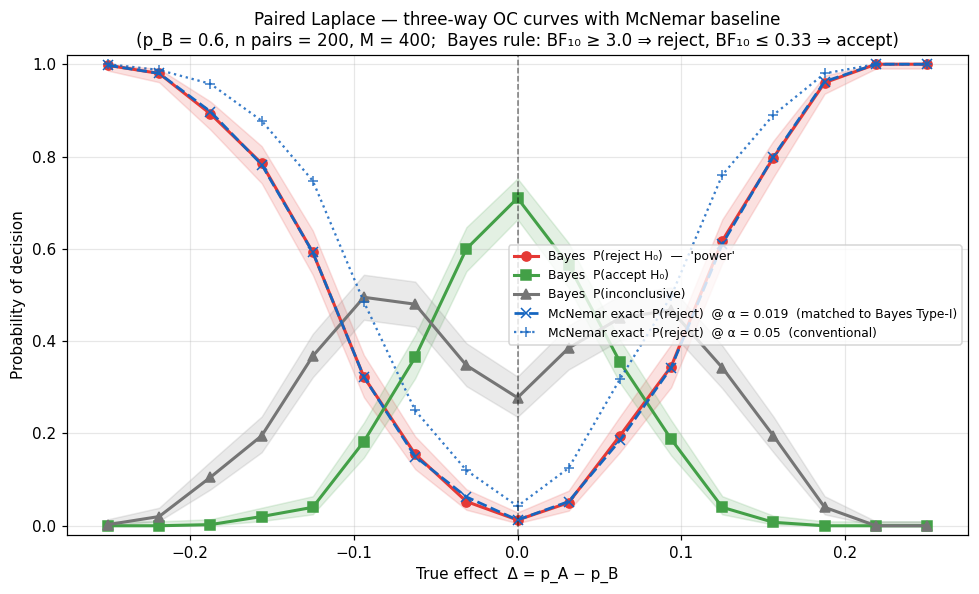
Plot 1 — Three-way OC curves with matched-α McNemar baseline

Bayesian P(reject H₀), P(accept H₀), P(inconclusive) as functions of the true effect Δ = p_A − p_B, with two McNemar overlays (α = 0.05 and the Bayes-matched α). Compared with the non-paired counterpart at the same (Δ, n), the paired reject curve is materially steeper — that's the variance reduction from pairing showing up in the operating characteristic.

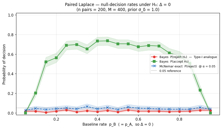
Plot 2 — Null-decision rates swept over the baseline rate

Type-I analogue. The Bayes P(reject H₀) curve under p_A = p_B = p, plus the McNemar α = 0.05 reference. The logit-scale prior on \(\delta_A\) is symmetric in logit space but its probability-scale projection is squeezed toward zero near the boundary, so the null curve is not flat across p.

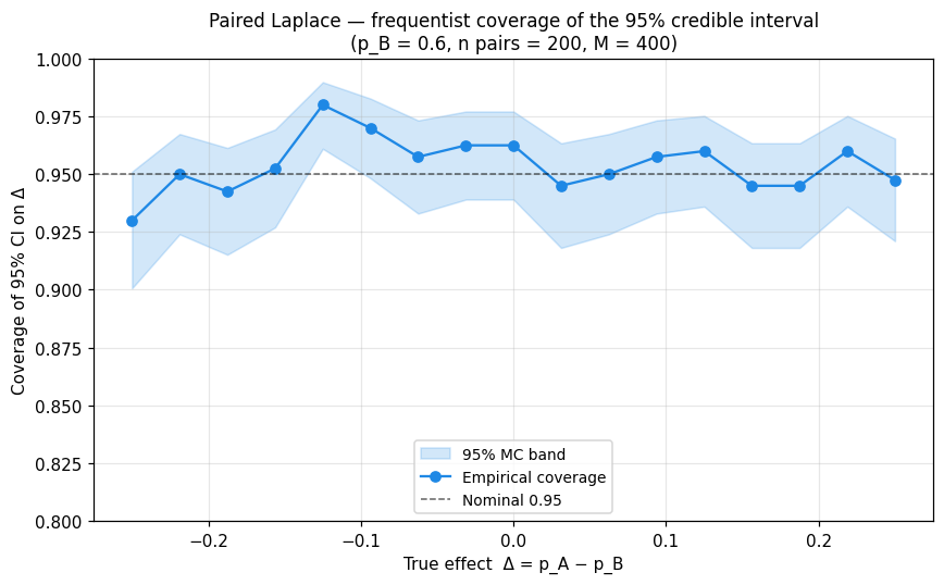
Plot 3 — Credible-interval coverage of Δ

Frequentist coverage of the 95 % equal-tailed posterior interval on Δ, derived from the Laplace posterior on \((\mu, \delta_A)\) pushed through \(\sigma(\mu + \delta_A) - \sigma(\mu)\). Should hover near the nominal 0.95 across the grid; deviations at extreme Δ are the regime where the second-order Laplace approximation starts to break down.

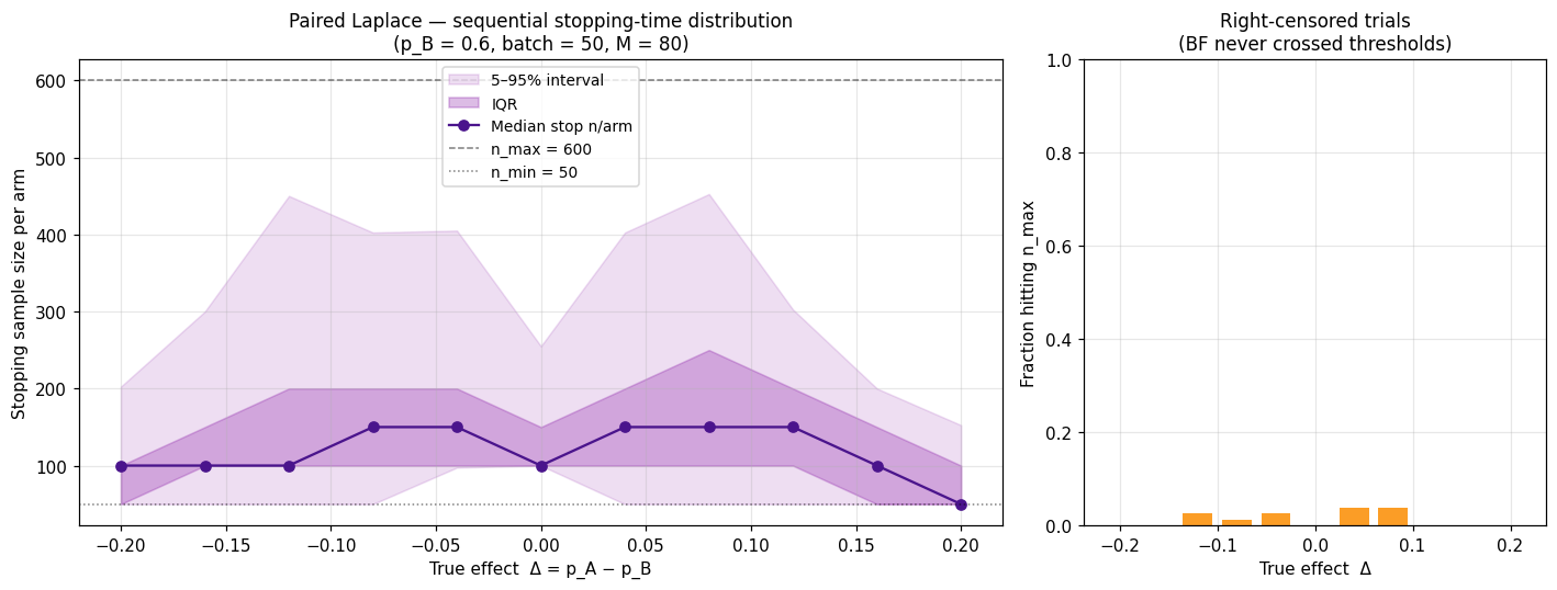
Plot 4 — Sequential stopping-time distribution

Median (and IQR / 5–95 % bands) of the per-arm stopping sample size of SequentialPairedBayesPropTest, as a function of the true effect. Trials that hit n_max are right-censored and reported separately. At decisive effects (|Δ| ≳ 0.15) the paired procedure typically stops in well under 200 pairs.

What can go wrong

The same failure modes as in the non-paired case apply, plus one paired-specific one:

• CI coverage drifts well off 0.95 → either the Laplace approximation is breaking (try a richer model or check the Newton solve converged) or the prior on \(\delta_A\) is biased for that part of the parameter space.
• The null-decision curve climbs above the nominal level → Type-I inflation under some p_B; consider a tighter \(\sigma_\delta\) or stricter BF thresholds.
• Asymmetric power around Δ = 0 → expected near boundary p_B because of the logit-scale prior; check the symmetry breaks line up with the prior's implicit asymmetry on the probability scale.
• Sequential censoring spikes → n_max is too low for the effect sizes you actually care about; raise it or relax the thresholds.

References

1. Rubin (1984). Bayesianly justifiable and relevant frequency calculations for the applied statistician. The Annals of Statistics, 12(4), 1151–1172.
2. Little (2006). Calibrated Bayes: A Bayes/frequentist roadmap. The American Statistician, 60(3), 213–223.
3. McNemar (1947). Note on the sampling error of the difference between correlated proportions or percentages. Psychometrika, 12(2), 153–157.
4. Brown, Cai & DasGupta (2001). Interval estimation for a binomial proportion. Statistical Science, 16(2), 101–133.

API

See API Reference — Operating Characteristics (Paired) for full function documentation.