Paired Model — Laplace Approximation
Overview
The paired model is used when both conditions are evaluated on the same items or subjects. It uses a Bernoulli logistic regression with a Laplace approximation (MAP + analytical Hessian) for fast, analytic posterior inference.
Two modes are supported:
- Fixed priors (default) — the prior scales \(\sigma_\mu\) and \(\sigma_\delta\) are user-chosen constants. The MAP is found by a 2-D Newton solver.
- Hierarchical (learned scales) — Inverse-Gamma hyperpriors are placed on \(\sigma_\mu^2\) and \(\sigma_\delta^2\), so the prior widths are learned from data via a 4-D Newton solver. This makes the Savage–Dickey Bayes factor robust to the Jeffreys–Lindley paradox.
Generative model
Fixed priors (default)
where \(\sigma(x) = 1/(1 + e^{-x})\) is the logistic sigmoid function. The parameter \(\delta_A\) captures group A's advantage on the logit scale; \(\mu\) is the shared baseline log-odds.
DAG (fixed priors)
graph TD
    sigma_mu(["σ_μ"]) --> mu["μ"]
    sigma_delta(["σ_δ"]) --> delta_A["δ_A"]

    mu --> pA["p_A = σ(μ + δ_A)"]
    delta_A --> pA
    mu --> pB["p_B = σ(μ)"]

    pA --> yA(["y_A,i"])
    pB --> yB(["y_B,i"])

    style sigma_mu fill:#e0e0e0,stroke:#757575
    style sigma_delta fill:#e0e0e0,stroke:#757575
    style mu fill:#bbdefb,stroke:#1565c0
    style delta_A fill:#bbdefb,stroke:#1565c0
    style pA fill:#c8e6c9,stroke:#2e7d32
    style pB fill:#c8e6c9,stroke:#2e7d32
    style yA fill:#fff9c4,stroke:#f9a825
    style yB fill:#fff9c4,stroke:#f9a825
Legend: grey = fixed hyperparameters, blue = latent parameters, green = deterministic, yellow = observed data.
Hierarchical logistic regression (learned scales)
When hyperprior_mu and hyperprior_delta are set, the model becomes a
hierarchical logistic regression where the prior variances are themselves
random variables:
DAG (hierarchical)
graph TD
    a_mu(["a_μ, b_μ"]) --> sigma2_mu["σ²_μ ~ IG"]
    a_delta(["a_δ, b_δ"]) --> sigma2_delta["σ²_δ ~ IG"]

    sigma2_mu --> mu["μ ~ N(0, σ²_μ)"]
    sigma2_delta --> delta_A["δ_A ~ N(0, σ²_δ)"]

    mu --> pA["p_A = σ(μ + δ_A)"]
    delta_A --> pA
    mu --> pB["p_B = σ(μ)"]

    pA --> yA(["y_A,i"])
    pB --> yB(["y_B,i"])

    style a_mu fill:#e0e0e0,stroke:#757575
    style a_delta fill:#e0e0e0,stroke:#757575
    style sigma2_mu fill:#ffe0b2,stroke:#e65100
    style sigma2_delta fill:#ffe0b2,stroke:#e65100
    style mu fill:#bbdefb,stroke:#1565c0
    style delta_A fill:#bbdefb,stroke:#1565c0
    style pA fill:#c8e6c9,stroke:#2e7d32
    style pB fill:#c8e6c9,stroke:#2e7d32
    style yA fill:#fff9c4,stroke:#f9a825
    style yB fill:#fff9c4,stroke:#f9a825
Legend: grey = fixed hyperparameters, orange = learned hyperparameters, blue = latent parameters, green = deterministic, yellow = observed data.
Laplace approximation
The Laplace method approximates the posterior as a multivariate Gaussian centred at the MAP (maximum a posteriori) estimate:
where \(\mathbf{H}\) is the Hessian of the negative log-posterior evaluated at the MAP.
Fixed-prior case (2-D)
Log-posterior
Let \(\boldsymbol{\theta} = (\mu, \delta_A)^\top\) denote the parameter vector. The log-posterior is
with \(p_A = \sigma(\mu + \delta_A)\) and \(p_B = \sigma(\mu)\).
Gradient
where \(k_A = \sum y_{A,i}\) and \(k_B = \sum y_{B,i}\).
Hessian of negative log-posterior
where \(w_A = p_A(1 - p_A)\) and \(w_B = p_B(1 - p_B)\), evaluated at the MAP.
Solver
The MAP is found by damped Newton iteration in 2-D using the closed-form gradient and Hessian above (no external optimizer is invoked). Unlike gradient descent, which only uses the gradient, Newton's method also uses the Hessian (second-derivative curvature) to compute the optimal step direction and size:
This solves the linear system \(\mathbf{H}\,\Delta\boldsymbol{\theta} = -\nabla f\) for the Newton step \(\Delta\boldsymbol{\theta}\). Because it accounts for curvature, Newton converges quadratically (the error squares each iteration) near the optimum, while gradient descent only converges linearly.
In the 2-D case the \(2\times 2\) system is solved in closed form via the cofactor inverse, and an Armijo backtracking line search guarantees monotone descent even from a poor starting point.
Because the negative log-posterior is strictly convex (Gaussian priors plus
Bernoulli likelihood), convergence is guaranteed. The
SequentialPairedBayesPropTest warm-starts each look from the
previous MAP, which typically requires only 1–3 iterations per update.
A warning is emitted if max_iter is reached without convergence.
Hierarchical case (4-D)
When Inverse-Gamma hyperpriors are placed on \(\sigma_\mu^2\) and \(\sigma_\delta^2\), the optimisation is lifted to a 4-D reparameterised space.
Reparameterisation
To enforce positivity of \(\sigma_\mu\) and \(\sigma_\delta\) we optimise in the log-scale parameterisation \(\psi_\mu = \log \sigma_\mu\) and \(\psi_\delta = \log \sigma_\delta\). The Jacobian of the transform is absorbed into the log-posterior, giving the 4-D parameter vector \(\boldsymbol{\phi} = (\mu,\, \delta_A,\, \psi_\mu,\, \psi_\delta)^\top\).
4-D negative log-posterior
Using the precision \(\tau = e^{-2\psi}\) (since \(\psi = \log\sigma\) implies \(\sigma^2 = e^{2\psi}\), so \(\tau = 1/\sigma^2 = e^{-2\psi}\)) and writing the Inverse-Gamma log-density on the \(\psi\)-scale:
where \(z_A = \mu + \delta_A\), \(z_B = \mu\), \(\tau_\mu = e^{-2\psi_\mu}\), \(\tau_\delta = e^{-2\psi_\delta}\).
4-D gradient
where \(r_A = k_A - n_A p_A\) and \(r_B = k_B - n_B p_B\) are the Bernoulli residuals.
4×4 Hessian (block-sparse)
with \(w_A = p_A(1-p_A)\), \(w_B = p_B(1-p_B)\).
Solver
The MAP is found by damped Newton iteration in 4-D using the closed-form gradient and Hessian above (no external optimizer is invoked). As in the 2-D case, Newton's method uses the Hessian to compute the optimal step direction and size:
This solves the linear system \(\mathbf{H}\,\Delta\boldsymbol{\phi} = -\nabla f\) for the Newton step \(\Delta\boldsymbol{\phi}\). Because it accounts for curvature, Newton converges quadratically near the optimum.
The \(4\times 4\) system is solved via numpy.linalg.solve, and an Armijo
backtracking line search guarantees monotone descent even from a poor
starting point. Convergence is checked by the \(\ell^\infty\)-norm of the
gradient; a warning is emitted if max_iter is reached without convergence.
Marginal posterior on \((\mu, \delta_A)\)
After convergence the full \(4\times 4\) Laplace covariance is
The marginal 2×2 covariance for \((\mu, \delta_A)\) is the top-left block \(\boldsymbol{\Sigma}_{2} = [\boldsymbol{\Sigma}_4]_{1:2,\,1:2}\), which already incorporates the additional uncertainty from learning \(\sigma_\mu\) and \(\sigma_\delta\). Samples from the Laplace posterior are drawn from \(\mathcal{N}\!\bigl(\hat{\boldsymbol{\theta}}_\text{MAP},\, \boldsymbol{\Sigma}_2\bigr)\).
Savage–Dickey Bayes factor (hierarchical)
Under the hierarchical model the marginal prior on \(\delta_A\) (after integrating out \(\sigma_\delta^2\)) is a Student-\(t\) distribution:
with \(\nu = 2a_\delta\) degrees of freedom and scale \(\sqrt{b_\delta / a_\delta}\). The Savage–Dickey ratio is therefore
When to use
- Fast inference — no MCMC, results in milliseconds
- Moderate sample sizes — works well with \(n \geq 30\)
- Exploratory analysis — quick iteration before committing to full MCMC
For exact posterior inference with convergence diagnostics, see Paired Model (Pólya-Gamma).
Step-by-step example
1. Simulate paired data
from bayesprop.resources.bayes_paired import PairedBayesPropTest
from bayesprop.utils.utils import simulate_paired_scores

sim = simulate_paired_scores(N=250, theta_A=0.69, theta_B=0.50, sigma_theta=0.0, seed=42)

print(f"True θ_A = {sim.theta_A:.2f},  θ_B = {sim.theta_B:.2f},  Δ = {sim.theta_A - sim.theta_B:.2f}")
print(f"Observed rates: A = {sim.y_A.mean():.3f},  B = {sim.y_B.mean():.3f}")
2. Fit the model
model = PairedBayesPropTest(
    prior_sigma_delta=1.0,
    seed=42,
    n_samples=50_000,
).fit(sim.y_A, sim.y_B)

s = model.summary
print(f"δ_A posterior mean = {s.delta_A_posterior_mean:+.4f}")
print(f"Mean Δ (prob)  = {s.mean_delta:+.4f}")
print(f"95% CI         = [{s.ci_95.lower:.4f}, {s.ci_95.upper:.4f}]")
print(f"P(A>B)         = {s.p_A_greater_B:.4f}")
3. Unified decision
d = model.decide()

print(f"Bayes Factor:  BF₁₀ = {d.bayes_factor.BF_10:.2f}  → {d.bayes_factor.decision}")
print(f"Posterior Null: P(H₀|D) = {d.posterior_null.p_H0:.4f}  → {d.posterior_null.decision}")
print(f"ROPE:          {d.rope.decision}  ({d.rope.pct_in_rope:.1%} in ROPE)")
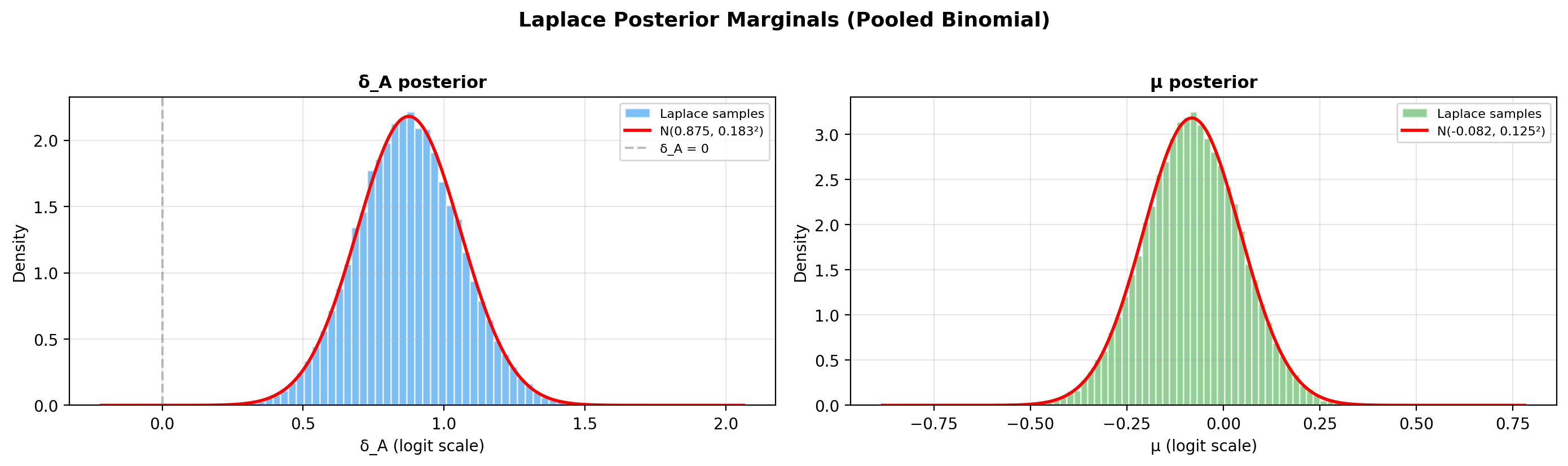
4. Posterior visualisation
The Laplace approximation produces a bivariate Gaussian in \((\mu, \delta_A)\). Use the built-in methods to inspect the implied probability posteriors \(p_A = \sigma(\mu + \delta_A)\), \(p_B = \sigma(\mu)\) and their difference \(\Delta = p_A - p_B\):
model.plot_posteriors()       # single-panel overlay of θ_A and θ_B
model.plot_posterior_delta()   # single-panel Δ = θ_A − θ_B on probability scale
If you need the raw MAP / covariance values for a custom plot, they are available on the fitted model:
import numpy as np

laplace = model.laplace
mu_map, delta_map = laplace["map"]
cov = laplace["cov"]
sd_m, sd_d = np.sqrt(cov[0, 0]), np.sqrt(cov[1, 1])

print(f"MAP: μ={mu_map:.4f}, δ_A={delta_map:.4f}")
print(f"Posterior sd: μ={sd_m:.4f}, δ_A={sd_d:.4f}")
print(f"Correlation: {cov[0, 1] / (sd_m * sd_d):.3f}")
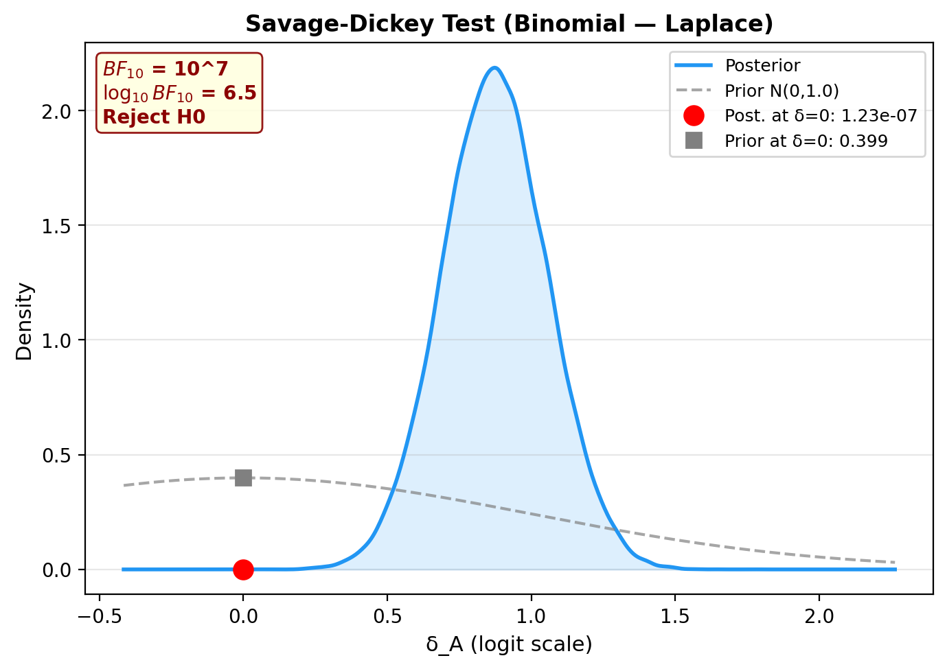
5. Savage-Dickey Bayes Factor plot
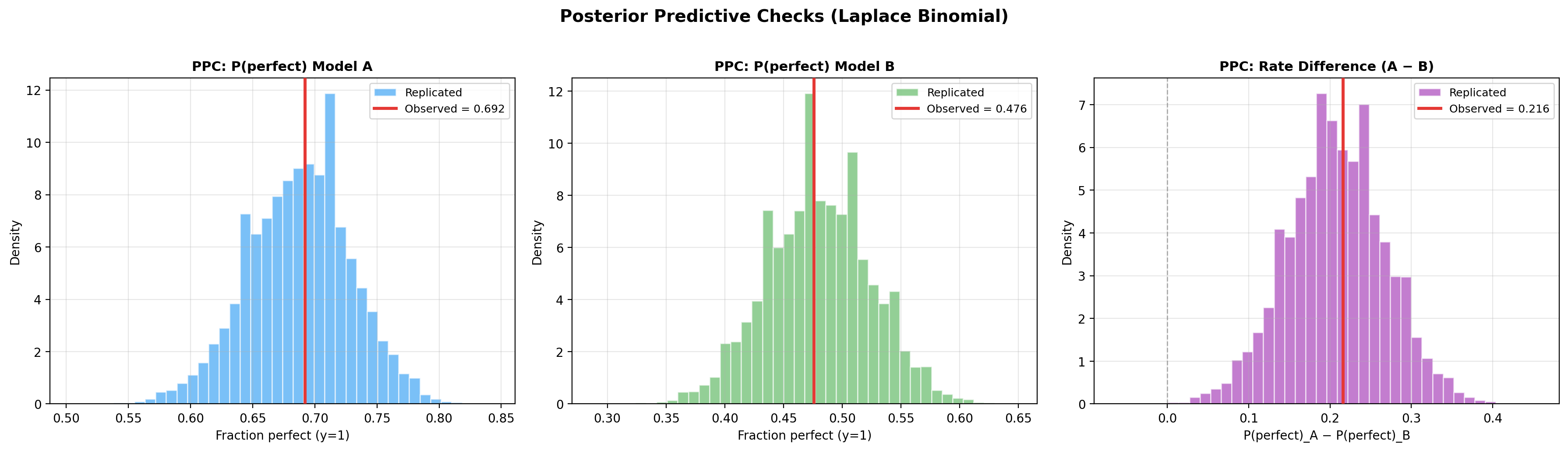
6. Posterior predictive checks
ppc = model.ppc_pvalues(seed=42)

print(f"{'Statistic':<20} {'Observed':>10} {'p-value':>10} {'Status':>10}")
print("-" * 55)
for stat_name, vals in ppc.items():
    print(f"{stat_name:<20} {vals.observed:>10.4f} {vals.p_value:>10.3f} {vals.status:>10}")
PPC plots (fraction perfect for each model + rate difference):
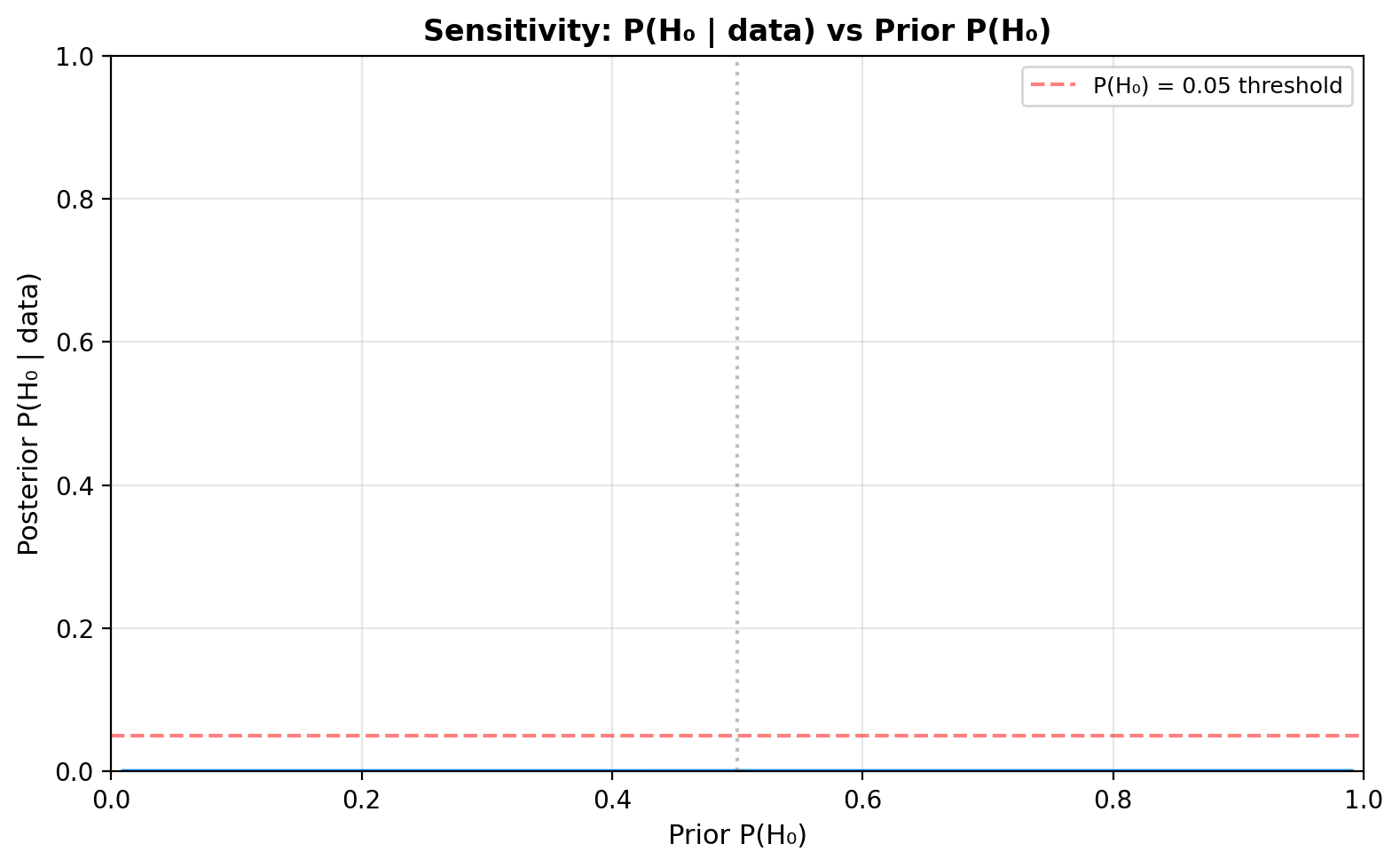
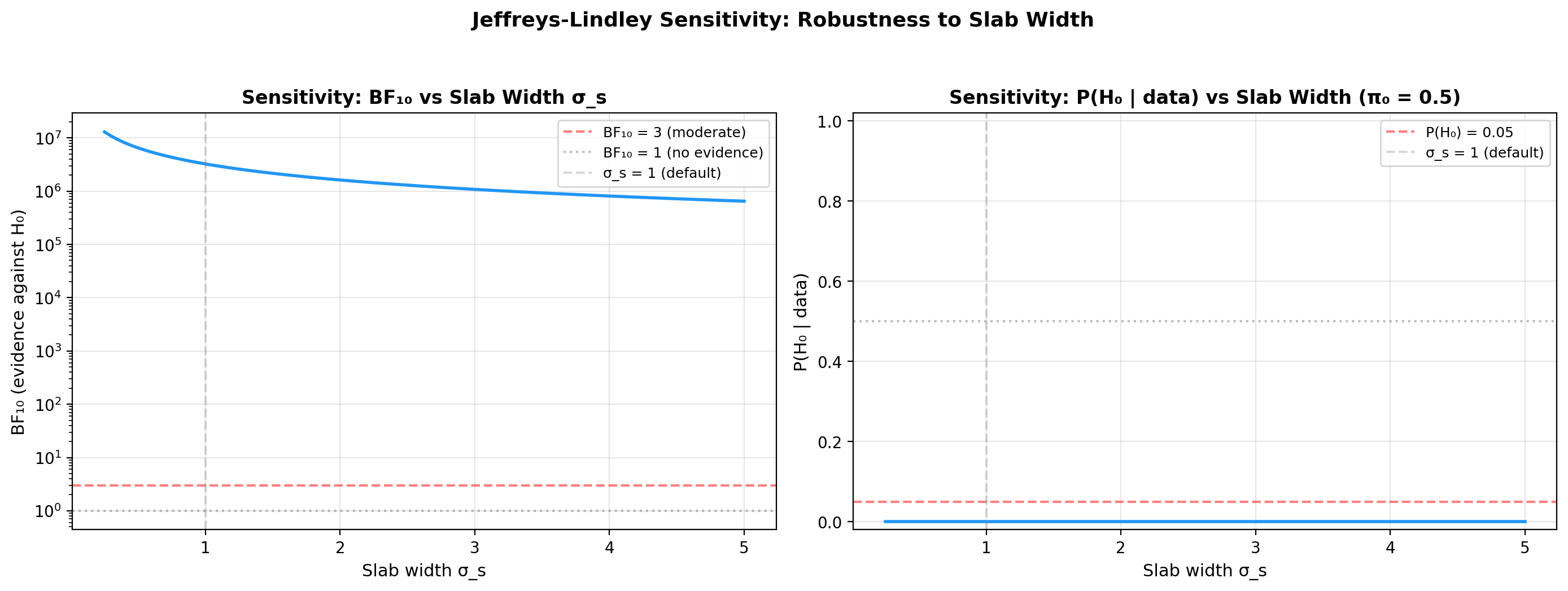
Prior sensitivity analysis
Sensitivity to prior P(H0)
Plot how the posterior \(P(H_0 \mid D)\) changes as you vary the prior \(\pi_0 = P(H_0)\):
Sensitivity to slab width sigma_s
The Savage-Dickey BF depends on the prior at \(\delta_A = 0\). For a
\(\mathcal{N}(0, \sigma_s)\) slab prior, a wider slab concentrates less
density at zero, inflating \(BF_{10}\). This is the Jeffreys-Lindley
paradox in action. The right panel of plot_sensitivity above already
sweeps \(\sigma_s\) on a log scale, so no extra code is needed:
Frequentist comparison (McNemar test)
For reference, you can compare the Bayesian result with McNemar's
exact test on the same paired binary data. The library ships a small
wrapper that returns a standardised
FrequentistTestResult:
from bayesprop.utils.utils import mcnemar_paired_test

freq = mcnemar_paired_test(model.y_A_obs, model.y_B_obs)
print(f"McNemar p = {freq.p_value:.4f},  discordant OR = {freq.odds_ratio}")
For a systematic Monte-Carlo evaluation of the paired Bayes rule's operating characteristics (Type-I rate, three-way decision curves, CI coverage, sequential stopping-time distribution) with a matched-α McNemar baseline overlay, see Frequentist Evaluation — Paired Laplace.
BFDA sample-size planning
from bayesprop.utils.utils import bfda_power_curve, plot_bfda_power

theta_A_hat = model.y_A_obs.mean()
theta_B_hat = model.y_B_obs.mean()
sample_sizes = [20, 30, 50, 75, 100, 150, 200, 300, 500]

power_curve = bfda_power_curve(
    theta_A_true=theta_A_hat,
    theta_B_true=theta_B_hat,
    sample_sizes=sample_sizes,
    design="paired",
    decision_rule="bayes_factor",
    bf_threshold=3.0,
    n_sim=200,
    seed=42,
)

plot_bfda_power(
    power_curve, theta_A_hat, theta_B_hat,
    title=f"BFDA Power Curve (Paired Laplace) — Δ = {theta_A_hat - theta_B_hat:.3f}"
)
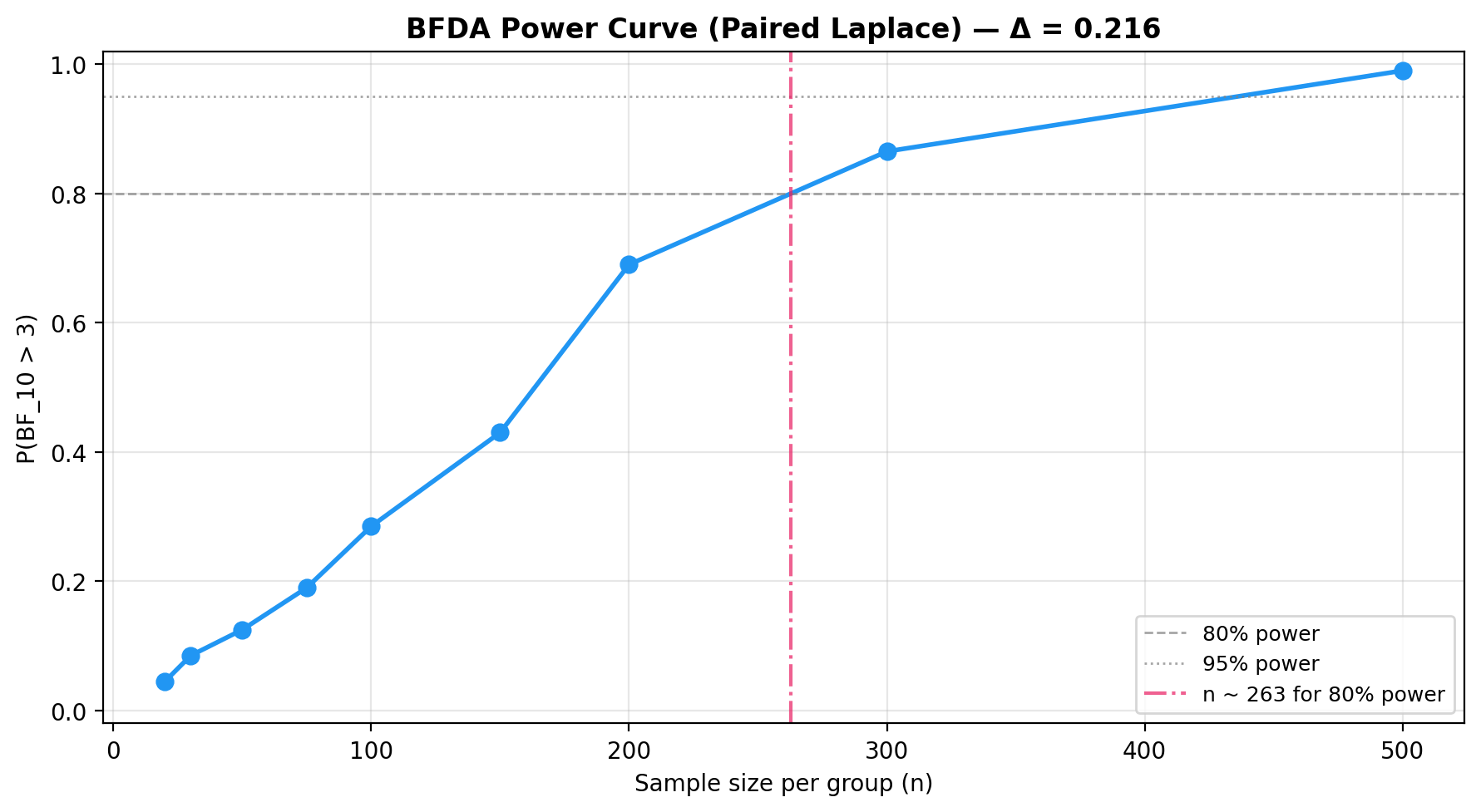
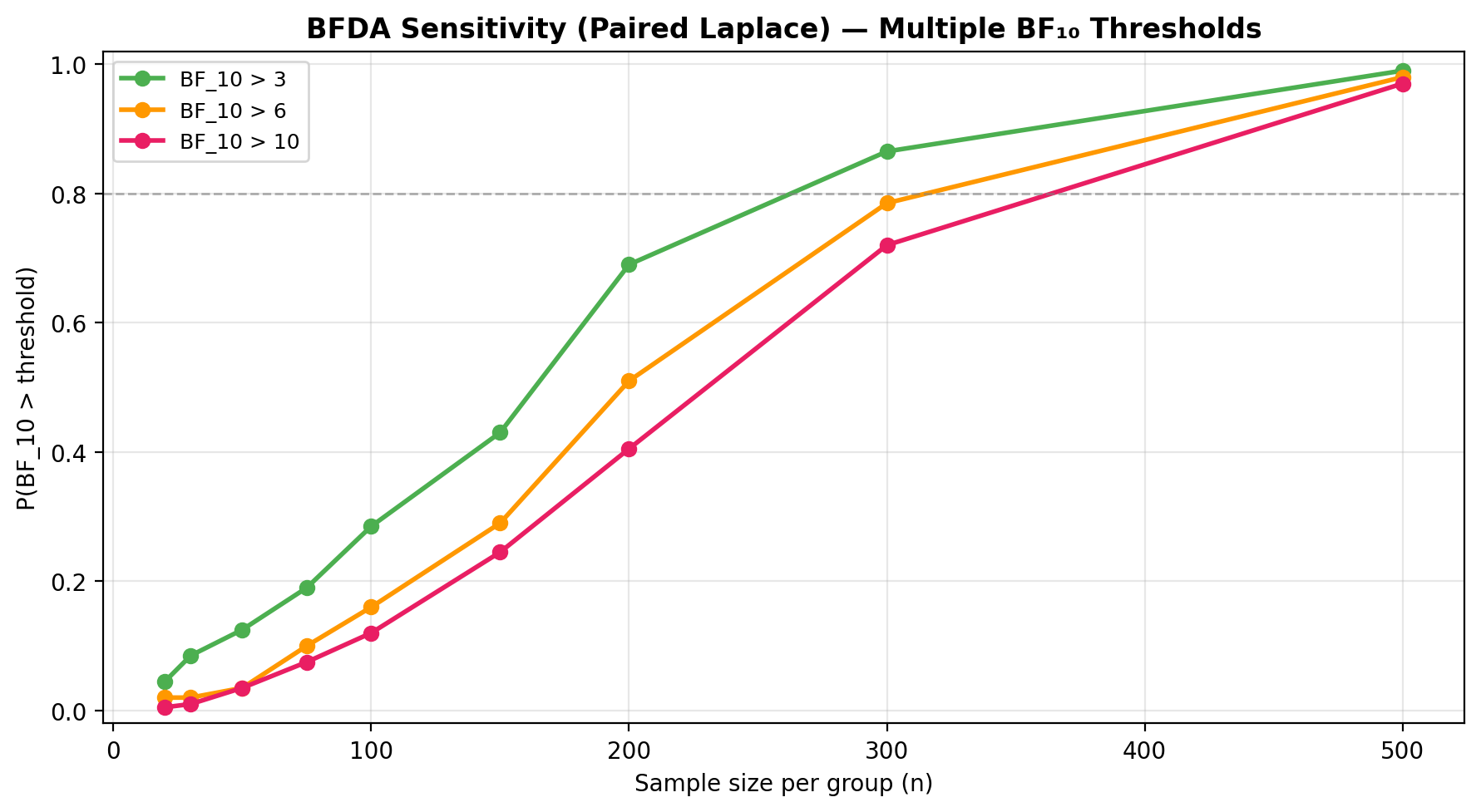
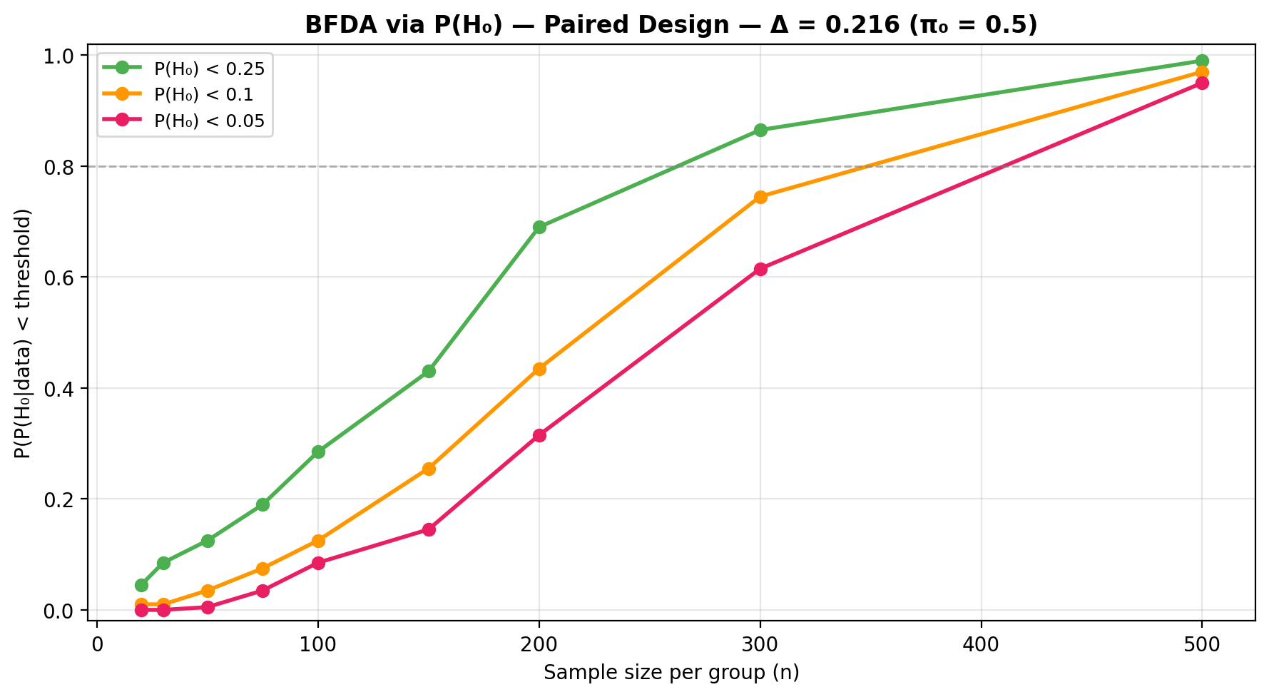
See the BFDA guide for sensitivity analysis and \(P(H_0)\)-based power curves.
Sequential design and decision making
In a sequential paired A/B test the binary observations arrive in batches over time and we update the Laplace posterior after each look. The pooled Bernoulli logistic likelihood depends on the data only through the four sufficient statistics \((n_A, k_A, n_B, k_B)\), so the cumulative counts carry all the information needed to recompute the Savage-Dickey Bayes factor on \(\delta_A = 0\), the posterior probability \(P(p_A > p_B)\) on the probability scale, and a ROPE decision at every look. Refitting on the running counts therefore yields exactly the same Laplace posterior as fitting all accumulated data in one shot — streaming introduces no additional approximation on top of the Laplace step itself.
Each refit is a damped Newton solve in 2D warm-started from the previous MAP, which typically converges in 1-3 iterations.
Stopping rule
At each look \(t\) the test evaluates the running \(\text{BF}_{10}^{(t)}\) and stops as soon as one of the following holds:
- \(\text{BF}_{10}^{(t)} \ge B_U\) (
bf_upper) -> stop for \(H_1\) (evidence of a difference). - \(\text{BF}_{10}^{(t)} \le B_L\) (
bf_lower) -> stop for \(H_0\) (evidence of practical equivalence). - \(\min(n_A^{(t)}, n_B^{(t)}) \ge n_{\max}\) -> stop because the budget is exhausted.
Because the Laplace posterior is a coherent likelihood-based object, optional stopping is permitted: performing many looks does not inflate a frequentist Type-I rate the way repeated \(p\)-values would.
Example: streaming paired Bernoulli batches
Ground truth on the logit scale: \(\mu = 0.5\), \(\delta_A = 0.6\). Each look delivers a batch of 25 paired observations.
import numpy as np
from bayesprop.resources.bayes_paired_laplace import SequentialPairedBayesPropTest

rng = np.random.default_rng(42)
p_A_true, p_B_true = 0.75, 0.62

def stream(n_batches: int = 40, batch_size: int = 25):
    for _ in range(n_batches):
        yield (
            rng.binomial(1, p_A_true, size=batch_size),
            rng.binomial(1, p_B_true, size=batch_size),
        )

seq = SequentialPairedBayesPropTest(
    prior_sigma_delta=1.0,
    bf_upper=10.0,
    bf_lower=0.1,
    n_max=1000,
)
final = seq.run(stream())

print("Stopped:", seq.stopped, "after", len(seq.history), "looks")
print("Reason :", seq.stop_reason)
Inspect the final snapshot and history
The last SequentialLaplaceLookResult exposes the same diagnostics as
the batch test (Laplace posterior state, \(P(p_A > p_B)\), Savage-Dickey
BF, ROPE), and history_frame() returns one row per look:
ps = final.posterior_state
print(f"MAP: mu={ps.mu_map:.4f}, delta_A={ps.delta_A_map:.4f}")
print(f"P(p_A > p_B) = {final.P_A_greater_B:.4f}")
print(f"BF10 = {final.decision.bayes_factor.BF_10:.3g}")
print(f"ROPE decision: {final.decision.rope.decision}")

df = seq.history_frame()       # per-look DataFrame
seq.plot_trajectory()           # BF10 and P(A>B) vs cumulative n
Equivalence to a single-shot fit
Because the Laplace posterior depends only on the cumulative
sufficient statistics, fitting all accumulated data in one shot yields
the same MAP and covariance as the sequential refit at the final
look — i.e. seq.last_model matches a PairedBayesPropTest().fit(...)
on the materialised cumulative arrays.
See the runnable notebook at
src/notebooks/sequential_paired_laplace_demo.ipynb for the full demo.
Hierarchical example
The hierarchical variant uses the same PairedBayesPropTest class — just
pass hyperprior_mu and hyperprior_delta (see the
generative model
and 4-D Laplace math above).
from bayesprop.resources.bayes_paired import PairedBayesPropTest
from bayesprop.utils.utils import simulate_paired_scores

sim = simulate_paired_scores(N=250, theta_A=0.69, theta_B=0.50, seed=42)

model = PairedBayesPropTest(
    hyperprior_mu=(3.0, 1.0),       # IG(3, 1) on σ²_μ
    hyperprior_delta=(3.0, 1.0),    # IG(3, 1) on σ²_δ
    seed=42,
    n_samples=50_000,
).fit(sim.y_A, sim.y_B)

model.print_summary()

d = model.decide()
print(f"BF₁₀ = {d.bayes_factor.BF_10:.2f}  →  {d.bayes_factor.decision}")
The fitted model stores the learned MAP prior scales:
laplace = model.laplace
print(f"Learned σ_μ (MAP)  = {laplace['sigma_mu_map']:.4f}")
print(f"Learned σ_δ (MAP)  = {laplace['sigma_delta_map']:.4f}")
print(f"Hierarchical mode: {laplace['hierarchical']}")
When to use the hierarchical variant
- You are unsure about a sensible value for \(\sigma_\delta\) and want the data to inform it rather than commit to a fixed slab width.
- You want a Bayes factor that is robust to the Jeffreys–Lindley paradox.
- You have enough data (\(n \gtrsim 50\)) for the 4-D Laplace to be accurate.
For a fixed-prior analysis where you deliberately choose \(\sigma_\delta\),
set hyperprior_mu=None, hyperprior_delta=None (the default).
Inputs and binarisation
Like the non-paired model, PairedBayesPropTest accepts both already-binary
{0, 1} inputs and continuous scores in [0, 1] (e.g. classifier
probabilities). Continuous inputs are auto-binarised at a configurable
threshold (default 0.5):
Values strictly outside [0, 1] or NaN raise ValueError instead of
being silently truncated — pass already-binarised arrays if you want the
fast path. The same threshold argument is exposed on
SequentialPairedBayesPropTest for streaming batches.
API
See API Reference — Paired Model (Laplace) for full method documentation.