Non-Paired Beta-Bernoulli Model
Overview
The non-paired model compares two independent groups using a conjugate Beta-Bernoulli model. Each group has its own success probability \(\theta_A\) and \(\theta_B\), estimated independently from binarized pass/fail data.
Use this model when group A and group B consist of independent observations (i.e. different items or subjects in each group).
Input arrays can be binary (0/1) or real-valued on (0, 1) — continuous scores are automatically binarized at a configurable threshold.
Generative model
Here \(\alpha_0\) and \(\beta_0\) are fixed hyperparameters (user-specified constants, not random variables). Although both groups share the same prior family, \(\theta_A\) and \(\theta_B\) are drawn independently, so the two groups are fully independent:
Dependence would only arise in a hierarchical model where \(\alpha_0, \beta_0\) are themselves random with a shared hyperprior. In this model they are fixed constants, so the DAG edges from \(\alpha_0, \beta_0\) to both \(\theta_A\) and \(\theta_B\) encode the same prior specification — not a probabilistic dependence path.
The posterior is available in closed form via conjugacy:
where \(k_A = \sum_{i} y_{A,i}\) is the number of successes (and analogously for group B).
Directed Acyclic Graph (DAG)
graph TD
    alpha0(["α₀"]) --> thetaA["θ_A"]
    beta0(["β₀"]) --> thetaA
    alpha0 --> thetaB["θ_B"]
    beta0 --> thetaB

    thetaA --> yA(["y_A,i"])
    thetaB --> yB(["y_B,j"])

    style alpha0 fill:#e0e0e0,stroke:#757575
    style beta0 fill:#e0e0e0,stroke:#757575
    style thetaA fill:#bbdefb,stroke:#1565c0
    style thetaB fill:#bbdefb,stroke:#1565c0
    style yA fill:#fff9c4,stroke:#f9a825
    style yB fill:#fff9c4,stroke:#f9a825
Legend: grey = hyperparameters, blue = latent parameters, yellow = observed data.
Posterior probability of superiority
A key quantity of interest is the probability that group A has a higher success rate than group B:
where \(f_{\theta_A \mid y}\) is the posterior density of \(\theta_A\) and \(F_{\theta_B \mid y}\) is the posterior CDF of \(\theta_B\).
Derivation
Because \(\theta_A\) and \(\theta_B\) are independent a posteriori:
Substituting the conjugate posteriors \(\theta_A \mid y \sim \text{Beta}(a_A, b_A)\) and \(\theta_B \mid y \sim \text{Beta}(a_B, b_B)\):
where \(I_x(a, b) = B(a,b)^{-1}\int_0^x t^{a-1}(1-t)^{b-1}\,\mathrm{d}t\) is the regularised incomplete Beta function.
Numerical evaluation
The integral is computed via Gauss-Legendre quadrature with \(n_q\) nodes on \([0, 1]\). The Beta density is evaluated in log-space for numerical stability:
where \((x_j, w_j)\) are the transformed quadrature nodes and weights on
\([0, 1]\). This gives a deterministic, exact result (up to
floating-point precision) — no Monte Carlo noise. The implementation
is in prob_greater in bayesprop.resources.bayes_nonpaired.
Difference posterior (exact convolution)
Distribution of a difference of independent random variables
Let \(X\) and \(Y\) be independent continuous random variables with densities \(f_X\) and \(f_Y\). The density of \(Z = X - Y\) is the convolution of \(f_X\) with the reflection of \(f_Y\):
This follows directly from the CDF:
Substituting \(y = x - z'\) and differentiating with respect to \(z\) yields the convolution integral above.
Application to the Beta posteriors
In our model the two posteriors are independent:
with \(a_A = \alpha_0 + k_A\), \(b_A = \beta_0 + n_A - k_A\) (and analogously for group B). Because both \(\theta_A\) and \(\theta_B\) have support \([0, 1]\), the difference \(\Delta = \theta_A - \theta_B\) has support \((-1, 1)\), and the integration limits tighten to:
The lower limit \(\max(0, z)\) ensures \(x \in [0,1]\); the upper limit \(\min(1, 1+z)\) ensures \(x - z \in [0,1]\).
Substituting the Beta densities:
where \(B(a, b) = \Gamma(a)\Gamma(b)/\Gamma(a+b)\) is the Beta function.
Closed form and numerical evaluation
Pham-Gia & Turkkan (1993) showed that the convolution integral admits a closed-form expression in terms of Appell's first hypergeometric function \(F_1(a;\,b_1,b_2;\,c;\,x,y)\), split by the sign of \(z\). However, the \(F_1\) arguments leave the double-series convergence region near \(z = 0\), requiring analytic continuation. In practice it is simpler (and equally exact) to evaluate the convolution integral directly via trapezoidal quadrature with the integrand computed in log-space for numerical stability:
This avoids underflow that would occur with direct multiplication of
many small values when the Beta parameters are large. The
implementation is in beta_diff_pdf in
bayesprop.resources.bayes_nonpaired.
Reference
Pham-Gia, T. & Turkkan, N. (1993). Bayesian analysis of the difference of two proportions. Communications in Statistics — Theory and Methods, 22(6), 1755–1771.
Properties
- Deterministic — no random sampling, so repeated calls yield identical results.
- Exact — no KDE bandwidth selection or MC noise; the only approximation is floating-point quadrature error (negligible in practice).
- Fast — evaluating \(f_\Delta(z)\) on a grid of 500 points takes a few milliseconds on modern hardware.
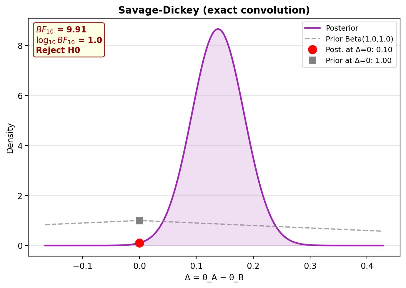
Savage-Dickey Bayes Factor
The hypothesis test \(H_0\!: \Delta = 0\) vs \(H_1\!: \Delta \neq 0\) uses the Savage-Dickey density ratio:
Both densities are computed via exact convolution (no KDE needed), so the Bayes factor is fully deterministic.
Step-by-step example
1. Simulate data
from bayesprop.utils.utils import simulate_nonpaired_scores
from bayesprop.resources.bayes_nonpaired import NonPairedBayesPropTest

sim = simulate_nonpaired_scores(N=150, theta_A=0.80, theta_B=0.75, seed=42)

print(f"True θ_A = {sim.theta_A:.2f},  θ_B = {sim.theta_B:.2f}")
print(f"True Δ   = {sim.theta_A - sim.theta_B:.2f}")
print(f"Observed rates: A = {sim.y_A.mean():.3f},  B = {sim.y_B.mean():.3f}")
2. Fit the model
model = NonPairedBayesPropTest(
    alpha0=1.0,      # Beta(1,1) = uniform prior
    beta0=1.0,
    seed=42,
    n_samples=50_000,
).fit(sim.y_A, sim.y_B)

s = model.summary
print(f"Mean Δ (θ_A − θ_B) = {s.mean_delta:+.4f}")
print(f"95% CI = [{s.ci_95.lower:.4f}, {s.ci_95.upper:.4f}]")
print(f"P(A > B) = {s.p_A_greater_B:.4f}")
Two estimators for P(A > B)
summary.p_A_greater_B uses Monte Carlo on the joint posterior
samples, while model.prob_greater() uses Gauss–Legendre
quadrature against the analytic Beta posteriors. Both estimate
the same probability and agree to MC error
(\(\sim 1/\sqrt{n_\text{samples}}\)); they will not, however, sum
to exactly 1 with prob_greater(reverse=True) because they come
from different estimators.
3. Unified decision (BF + P(H₀) + ROPE)
d = model.decide()

print(f"Bayes Factor:  BF₁₀ = {d.bayes_factor.BF_10:.2f}  → {d.bayes_factor.decision}")
print(f"Posterior Null: P(H₀|D) = {d.posterior_null.p_H0:.4f}  → {d.posterior_null.decision}")
print(f"ROPE:          {d.rope.decision}  ({d.rope.pct_in_rope:.1%} in ROPE)")
Bayes Factor:  BF₁₀ = 9.91  → Reject H0
Posterior Null: P(H₀|D) = 0.0917  → Undecided
ROPE:          Reject H0 — A practically better  (0.6% in ROPE)
\(BF_{10}=9.91\) sits at the upper edge of "moderate" on Jeffreys' scale
(\(BF_{10}=10\) is the boundary to "strong"); a longer MC run
(n_samples=100_000) can nudge it across.
4. Plot posteriors
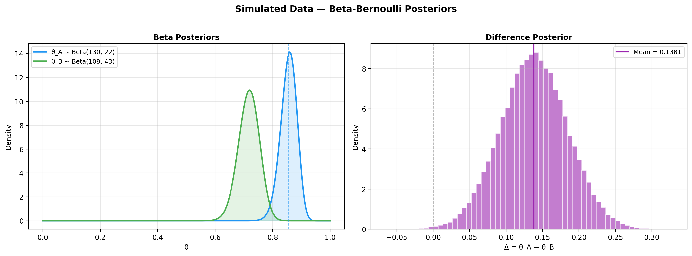
5. Savage-Dickey plot
6. Posterior predictive checks
ppc = model.ppc_pvalues(seed=42)

print(f"{'Statistic':<25} {'Observed':>10} {'p-value':>10} {'Status':>8}")
print("-" * 55)
for stat, vals in ppc.items():
    print(f"{stat:<25} {vals.observed:>10.4f} {vals.p_value:>10.3f} {vals.status:>8}")
Statistic                   Observed    p-value   Status
-------------------------------------------------------
mean(y_A)                     0.8600      0.953       OK
mean(y_B)                     0.7200      0.974       OK
mean(y_A)-mean(y_B)           0.1400      0.979       OK
A p-value \(< 0.05\) flags that the observed statistic is extreme under the fitted model (potential misfit); \(> 0.05\) means the model reproduces that aspect of the data adequately. The two-sided p-value uses the mid-p convention (ties at \(T^{\text{rep}}=T^{\text{obs}}\) are split evenly between the two tails) so it does not clip at 1.0 on discrete data.
Saturated model — interpret with care
For the conjugate Beta-Bernoulli model the sample mean is a sufficient statistic for each group, so PPC checks based on the means (and any deterministic function of them, including the sample variance for binary data) are guaranteed to be close to the centre of the replicated distribution. P-values near 1.0 are therefore expected here and do not constitute a strong test of fit — they only catch gross misspecification (e.g. wrong likelihood family). Meaningful PPC requires either covariates or a hierarchical structure that the sample mean does not summarise.
Prior sensitivity analysis
Test how results change with different priors to check robustness:
priors = [
    ("Uniform Beta(1,1)",      1.0, 1.0),
    ("Jeffreys Beta(0.5,0.5)", 0.5, 0.5),
    ("Informative Beta(2,2)",  2.0, 2.0),
    ("Strong Beta(5,5)",       5.0, 5.0),
]

print(f"{'Prior':<28} {'BF₁₀':>8} {'BF Decision':<20} {'ROPE Decision':<20}")
print("=" * 80)

for name, a0, b0 in priors:
    m = NonPairedBayesPropTest(alpha0=a0, beta0=b0, seed=42, n_samples=50_000).fit(y_A, y_B)
    d_i = m.decide()
    print(f"{name:<28} {d_i.bayes_factor.BF_10:>8.2f} "
          f"{d_i.bayes_factor.decision:<20} {d_i.rope.decision:<20}")
If the conclusion is stable across priors, you can be confident the result is not an artifact of the prior choice.
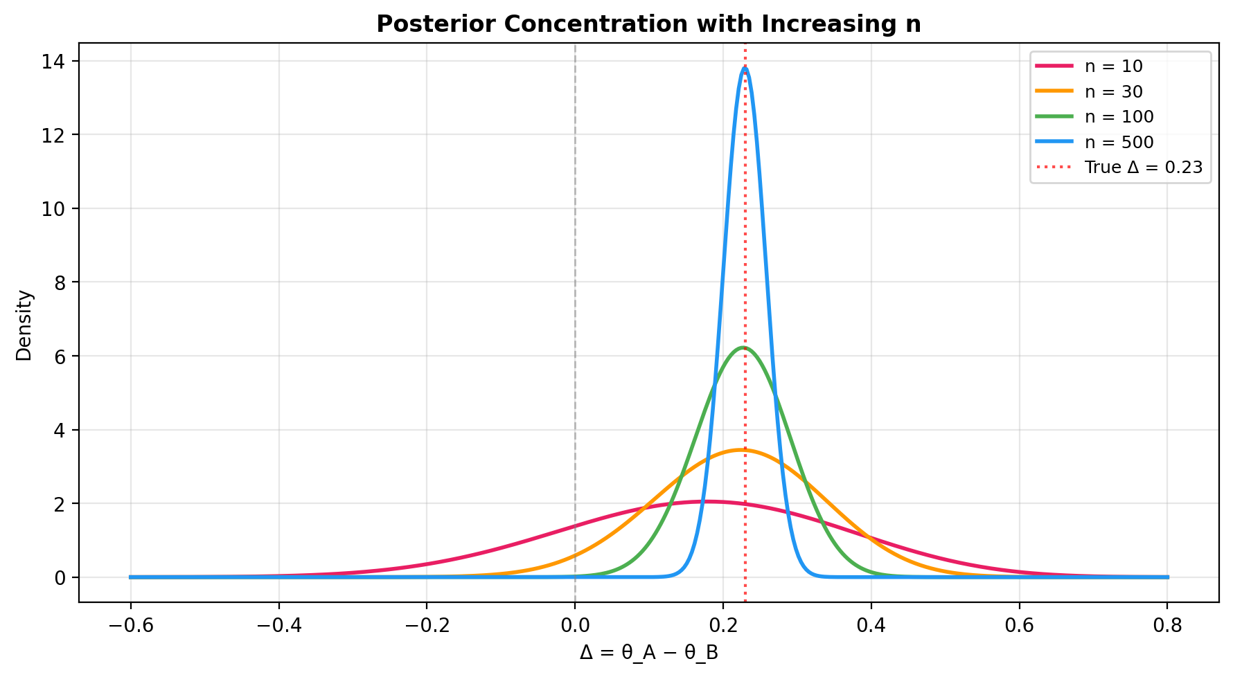
Posterior concentration with increasing n
As the sample size grows, the posterior of \(\Delta\) concentrates around the true effect size. This plot shows how precision improves:
import numpy as np
import matplotlib.pyplot as plt
from bayesprop.resources.bayes_nonpaired import beta_diff_pdf

z_grid = np.linspace(-0.6, 0.8, 400)
fig, ax = plt.subplots(figsize=(9, 5))

for n, col in zip([10, 30, 100, 500], ["#E91E63", "#FF9800", "#4CAF50", "#2196F3"]):
    a_A = 1 + int(0.78 * n)
    b_A = 1 + n - int(0.78 * n)
    a_B = 1 + int(0.55 * n)
    b_B = 1 + n - int(0.55 * n)
    density = np.array([beta_diff_pdf(z, a_A, b_A, a_B, b_B) for z in z_grid])
    ax.plot(z_grid, density, color=col, linewidth=2, label=f"n = {n}")

ax.axvline(0.23, color="red", linestyle=":", linewidth=1.5, alpha=0.7, label="True Δ = 0.23")
ax.axvline(0, color="gray", linestyle="--", linewidth=1, alpha=0.5)
ax.set_xlabel("Δ = θ_A − θ_B")
ax.set_ylabel("Density")
ax.set_title("Posterior Concentration with Increasing n")
ax.legend(fontsize=9)
ax.grid(alpha=0.3)
plt.tight_layout()
plt.show()
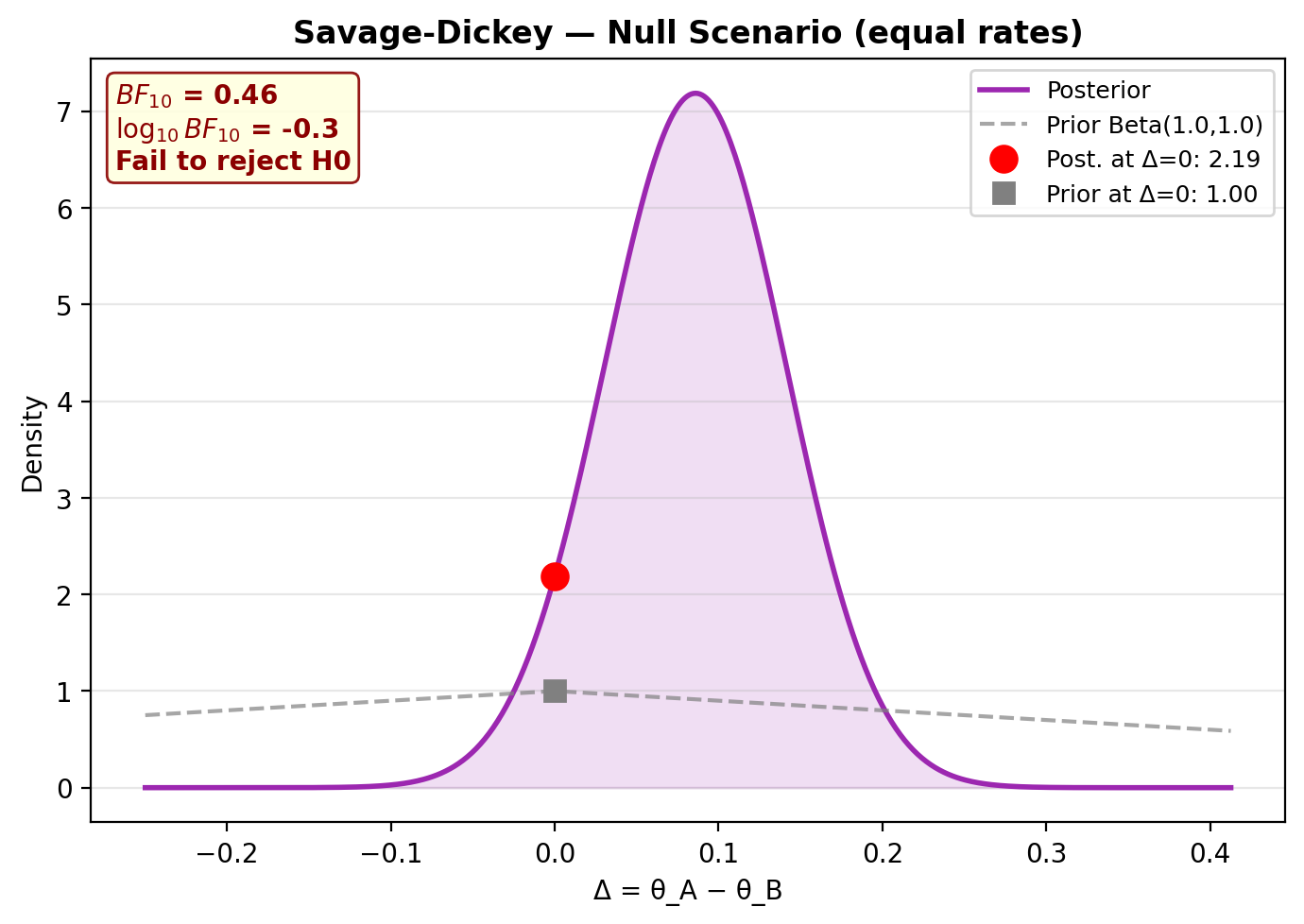
Null scenario (equal rates)
Under the null (\(\theta_A = \theta_B\)), the model should correctly find \(BF_{01} > 1\) (evidence for \(H_0\)):
rng_null = np.random.default_rng(99)
y_A_null = rng_null.binomial(1, 0.65, size=150).astype(float)
y_B_null = rng_null.binomial(1, 0.65, size=150).astype(float)

model_null = NonPairedBayesPropTest(seed=99, n_samples=50_000).fit(y_A_null, y_B_null)
model_null.print_summary()
model_null.plot_savage_dickey(title="Savage-Dickey — Null Scenario (equal rates)")
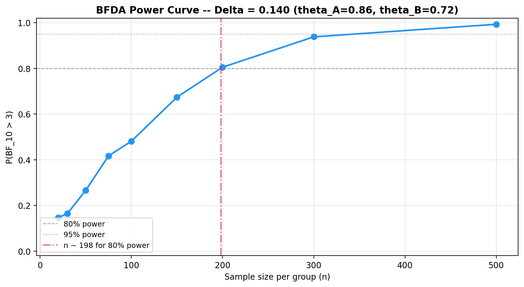
BFDA sample-size planning
Use Bayes Factor Design Analysis to determine how many observations you need for a given effect size. See the BFDA guide for details.
from bayesprop.utils.utils import bfda_power_curve, plot_bfda_power

theta_A_hat = y_A.mean()
theta_B_hat = y_B.mean()

sample_sizes = [20, 30, 50, 75, 100, 150, 200, 300, 500]

power_curve = bfda_power_curve(
    theta_A_true=theta_A_hat,
    theta_B_true=theta_B_hat,
    sample_sizes=sample_sizes,
    design="nonpaired",
    decision_rule="bayes_factor",
    bf_threshold=3.0,
    n_sim=1000,
    seed=42,
)

plot_bfda_power(power_curve, theta_A_hat, theta_B_hat)
Sequential design and decision making
In a sequential A/B test the data arrive in batches over time and we update the posterior after each look. Because the Beta–Bernoulli model is conjugate, the running posterior
acts as the prior for the next batch. Four sufficient statistics per arm therefore carry all the information needed to recompute the Savage–Dickey Bayes factor on \(\Delta = \theta_A - \theta_B\), the posterior probability \(P(\theta_B > \theta_A)\), and a ROPE decision at every look.
Stopping rule
At each look \(t\) the test evaluates the running \(\text{BF}_{10}^{(t)}\) and stops as soon as one of the following holds:
- \(\text{BF}_{10}^{(t)} \ge B_U\) (
bf_upper) → stop for \(H_1\) (evidence of a difference). - \(\text{BF}_{10}^{(t)} \le B_L\) (
bf_lower) → stop for \(H_0\) (evidence of practical equivalence). - \(\min(n_A^{(t)}, n_B^{(t)}) \ge n_{\max}\) → stop because the budget is exhausted.
A minimum sample size \(n_{\min}\) per arm (n_min) is enforced before any BF-based
stop is allowed, which avoids unstable early Bayes factors. Because the
posterior is exact and conjugate, performing many looks does not inflate
a frequentist Type-I rate the way repeated \(p\)-values would: the BF is a
coherent likelihood ratio whose interpretation is invariant to the stopping
rule (optional stopping is permitted).
Example: streaming Bernoulli batches
Ground truth \(\theta_A = 0.75\), \(\theta_B = 0.55\) (\(\Delta = 0.20\) in favour of A). Each look delivers a batch of 25 Bernoulli observations per arm.
import numpy as np
from bayesprop.resources.bayes_nonpaired import SequentialNonPairedBayesPropTest

rng = np.random.default_rng(42)
theta_A_true, theta_B_true = 0.75, 0.55
batch_size = 25
n_batches_max = 40

def stream():
    """Yield (y_a_batch, y_b_batch) pairs of binary observations."""
    for _ in range(n_batches_max):
        y_a = rng.binomial(1, theta_A_true, size=batch_size).astype(float)
        y_b = rng.binomial(1, theta_B_true, size=batch_size).astype(float)
        yield y_a, y_b

seq = SequentialNonPairedBayesPropTest(
    alpha0=1.0,
    beta0=1.0,
    bf_upper=10.0,
    bf_lower=0.1,
    n_min=30,
    n_max=1000,
    rope_epsilon=0.02,
    seed=0,
    n_samples=10_000,
    verbose=True,
)

final = seq.run(stream())

print("Stopped:", seq.stopped)
print("Reason :", seq.stop_reason)
print("Looks  :", len(seq.history))
print("Final n per arm:", final.n_A, final.n_B)
Typical output:
[look 1] n_A=25  n_B=25  P(B>A)=0.800 BF10=0.478 stop=False
[look 2] n_A=50  n_B=50  P(B>A)=0.338 BF10=0.254 stop=False
[look 3] n_A=75  n_B=75  P(B>A)=0.244 BF10=0.240 stop=False
[look 4] n_A=100 n_B=100 P(B>A)=0.118 BF10=0.336 stop=False
[look 5] n_A=125 n_B=125 P(B>A)=0.017 BF10=1.43  stop=False
[look 6] n_A=150 n_B=150 P(B>A)=0.003 BF10=6.99  stop=False
[look 7] n_A=175 n_B=175 P(B>A)=0.000 BF10=187   stop=True   (BF10 ≥ 10.0)

Stopped: True
Reason : BF10 ≥ 10.0 (evidence for H1)
Looks  : 7
Final n per arm: 175 175
Inspect the final snapshot and history
The last SequentialLookResult exposes the same diagnostics as the batch
test (posterior state, \(P(\theta_B > \theta_A)\), Savage–Dickey BF, ROPE),
and history_frame() returns one row per look:
ps = final.posterior_state
print(f"theta_A | data ~ Beta({ps.alpha_A:.0f}, {ps.beta_A:.0f})")
print(f"theta_B | data ~ Beta({ps.alpha_B:.0f}, {ps.beta_B:.0f})")
print(f"P(theta_B > theta_A) = {final.P_B_greater_A:.4f}")
print(f"BF10 = {final.decision.bayes_factor.BF_10:.3g}")
print(f"ROPE decision: {final.decision.rope.decision}")

df = seq.history_frame()       # per-look DataFrame
seq.plot_trajectory()           # BF10 and P(B>A) vs cumulative n
Equivalence to a single-shot fit
Because of conjugacy, fitting all accumulated data in one shot must yield exactly the same posterior as the sequential update — a useful sanity check:
from bayesprop.resources.bayes_nonpaired import NonPairedBayesPropTest

y_a_all = np.r_[np.ones(final.successes_A), np.zeros(final.n_A - final.successes_A)]
y_b_all = np.r_[np.ones(final.successes_B), np.zeros(final.n_B - final.successes_B)]

bb_batch = NonPairedBayesPropTest(alpha0=1.0, beta0=1.0, seed=0, n_samples=10_000).fit(
    y_a_all, y_b_all
)
# bb_batch.a_A, bb_batch.b_A, ... match seq.posterior_state exactly.
See the runnable notebook at
src/notebooks/sequential_nonpaired_demo.ipynb for the full demo.
API
See API Reference — Non-Paired Model for full method documentation.