Frequentist Evaluation

A Bayesian model doesn't have a Type-I error, but the moment we wrap it in a decision rule — e.g. "reject \(H_0\) if \(BF_{10} \geq 3\), accept if \(BF_{10} \leq 1/3\), otherwise inconclusive" — the rule is a function from data to a decision and therefore has well-defined frequentist operating characteristics. Estimating those by Monte-Carlo simulation is the standard calibrated Bayes check (Rubin 1984; Little 2006).

This page is about evaluating the chosen procedure after you've fixed its parameters. For the complementary question — how do I pick the sample size in the first place? — see BFDA. For the paired analogue (Laplace approximation + McNemar baseline) see Frequentist Evaluation — Paired Laplace.

What to estimate

Four diagnostics together replace a single "power curve" — the power curve is the wrong object for a Bayesian rule because it cannot represent the inconclusive zone:

Diagnostic	What it answers
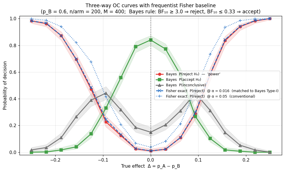
Three-way OC	P(reject H₀), P(accept H₀), P(inconclusive) as functions of the true effect Δ = p_A − p_B
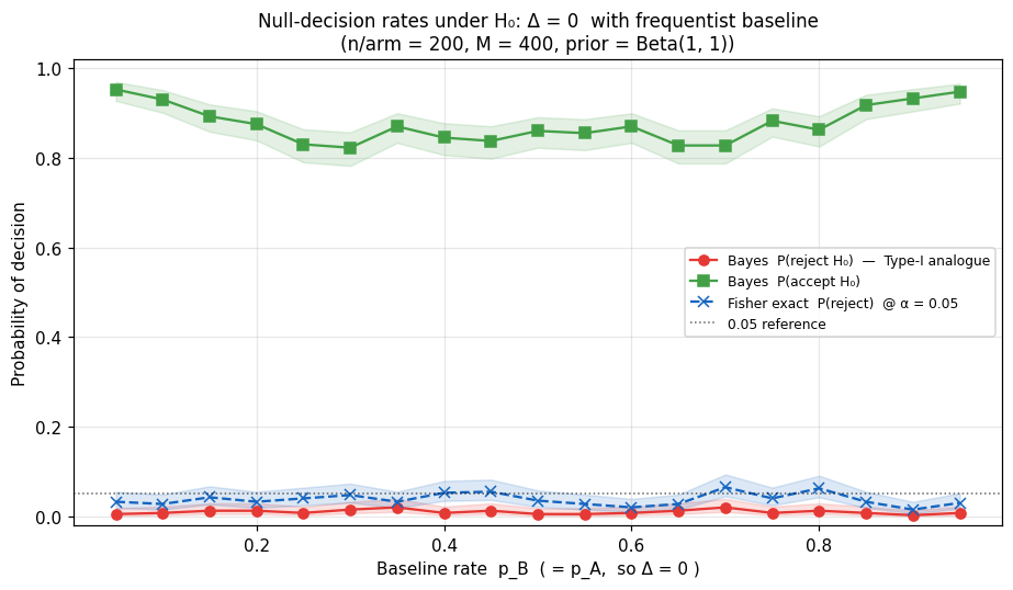
Null-decision sweep	P(reject H₀ \| Δ = 0) swept over the baseline rate p_B (BFs on proportions are not translation-invariant in p)
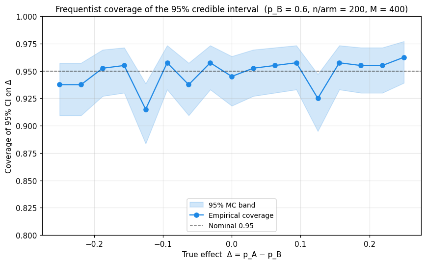
CI coverage	Frequentist coverage of the 95 % credible interval on Δ
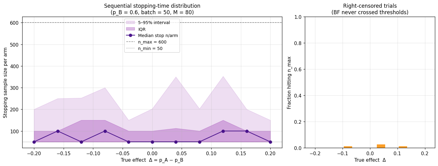
Sequential stopping-time distribution	Empirical distribution of the per-arm sample size at which SequentialNonPairedBayesPropTest stops

Three-way decision classifier

Use classify_bf so the simulated OC analysis and the deployed sequential procedure share one decision boundary:

from bayesprop.resources.bayes_nonpaired import classify_bf

bf10 = model.fit(y_A, y_B).savage_dickey_test().BF_10
category = classify_bf(bf10, bf_upper=3.0, bf_lower=1.0 / 3.0)
# → "reject" | "accept" | "inconclusive"

See Decision Rules → Three-way classification for the threshold conventions.

Frequentist baseline (Fisher's exact)

For a like-for-like comparison against a classical test, run Fisher's exact two-proportion test on the same simulated data:

from bayesprop.utils.utils import (
    fisher_exact_nonpaired_test,
    simulate_nonpaired_scores,
)

sim = simulate_nonpaired_scores(N=200, theta_A=0.75, theta_B=0.60)
freq = fisher_exact_nonpaired_test(sim.y_A, sim.y_B)
print(f"Fisher p = {freq.p_value:.4f},  OR = {freq.odds_ratio:.3f}")

This is most useful as a calibration reference for OC plots: pick a frequentist α such that the empirical Type-I rate at Δ = 0 matches the Bayes BF rule's Type-I rate, then overlay the two power curves. If the matched-α frequentist curve tracks the Bayes P(reject H₀) curve closely, the Bayes procedure is paying nothing in efficiency for the bonus of an explicit P(accept H₀) zone.

Pre-built OC simulation harness

The full simulation logic — grid sweeps for the three-way OC plot, matched-α calibration, CI coverage tracking, Wilson Monte-Carlo bands and the sequential stopping-time distribution — lives in bayesprop.utils.operation_characteristics. The notebook src/notebooks/operating_characteristics_nonpaired.ipynb is a thin orchestration layer on top of it, so you can call the same functions directly from your own scripts:

import numpy as np
from bayesprop.utils.operation_characteristics import (
    grid_fixed_n,
    matched_calibration_alpha,
    simulate_sequential,
    wilson_band,
)

grid = [(round(0.6 + d, 4), 0.6) for d in np.linspace(-0.2, 0.2, 11)]
df_oc, pvals = grid_fixed_n(
    grid, n=200, n_sim=400, seed=20260514,
    alpha0=1.0, beta0=1.0, bf_upper=3.0, bf_lower=1.0 / 3.0,
)
idx_null = int(np.argmin(np.abs(df_oc["delta"])))
alpha_matched = matched_calibration_alpha(
    pvals, df_oc.iloc[idx_null]["reject"], idx_null,
)
lo, hi = wilson_band(df_oc["reject"].to_numpy(), n_sim=400)

seq = simulate_sequential(
    p_A=0.75, p_B=0.55, n_sim=80, rng=np.random.default_rng(0),
    n_min=50, n_max=600, batch_size=50,
)

See API → Operating Characteristics for the full reference.

Worked example — the four diagnostic plots

The plots below are produced end-to-end by the notebook above with p_B = 0.6, n_per_arm = 200, M = 400 replicates, prior Beta(1, 1), and BF thresholds (3, 1/3). Shaded bands are 95 % Wilson Monte-Carlo bands.

Plot 1 — Three-way OC curves with matched-α frequentist baseline

Bayesian P(reject H₀), P(accept H₀), P(inconclusive) as functions of the true effect Δ = p_A − p_B, with two Fisher overlays (α = 0.05 and the Bayes-matched α).

Plot 2 — Null-decision rates swept over the baseline rate

Type-I analogue. The Bayes P(reject H₀) curve under p_A = p_B = p, plus the Fisher α = 0.05 reference. Because BFs on proportions are not translation-invariant in p, it pays to look at the whole curve, not just at p = 0.5.

Plot 3 — Credible-interval coverage of Δ

Frequentist coverage of the 95 % equal-tailed posterior interval on Δ. Should hover near the nominal 0.95 across the grid; small deviations near the boundaries (p_A near 0 or 1) are expected.

Plot 4 — Sequential stopping-time distribution

Median (and IQR / 5–95 % bands) of the per-arm stopping sample size of SequentialNonPairedBayesPropTest, as a function of the true effect. Trials that hit n_max are right-censored and reported separately.

What can go wrong

These plots are a quick health check on the procedure. Typical failure modes a regression will surface:

• CI coverage drifts well off 0.95 → prior / likelihood combination is biased somewhere in the parameter space.
• The null-decision curve climbs above the nominal level → Type-I inflation under some p_B; consider stricter BF thresholds.
• Asymmetric power around Δ = 0 → the procedure (or the prior) is not symmetric in the way you expected.
• Sequential censoring spikes → n_max is too low for the effect sizes you actually care about; raise it or relax the thresholds.

References

1. Rubin (1984). Bayesianly justifiable and relevant frequency calculations for the applied statistician. The Annals of Statistics, 12(4), 1151–1172.
2. Little (2006). Calibrated Bayes: A Bayes/frequentist roadmap. The American Statistician, 60(3), 213–223.
3. Brown, Cai & DasGupta (2001). Interval estimation for a binomial proportion. Statistical Science, 16(2), 101–133.

API

See API Reference — Operating Characteristics for full function documentation.