Paired Model — Pólya-Gamma Gibbs Sampler
Overview
This model uses the same paired logistic regression as the Laplace variant, but performs exact posterior inference via Pólya-Gamma data augmentation and Gibbs sampling. It provides multi-chain MCMC diagnostics (R-hat, ESS) to verify convergence.
Generative model
Directed Acyclic Graph (DAG)
graph TD
    sigma_mu(["σ_μ"]) --> mu["μ"]
    sigma_delta(["σ_δ"]) --> delta_A["δ_A"]

    mu --> pA["p_A = σ(μ + δ_A)"]
    delta_A --> pA
    mu --> pB["p_B = σ(μ)"]

    pA --> yA(["y_A,i"])
    pB --> yB(["y_B,i"])

    style sigma_mu fill:#e0e0e0,stroke:#757575
    style sigma_delta fill:#e0e0e0,stroke:#757575
    style mu fill:#bbdefb,stroke:#1565c0
    style delta_A fill:#bbdefb,stroke:#1565c0
    style pA fill:#c8e6c9,stroke:#2e7d32
    style pB fill:#c8e6c9,stroke:#2e7d32
    style yA fill:#fff9c4,stroke:#f9a825
    style yB fill:#fff9c4,stroke:#f9a825
Legend: grey = hyperparameters, blue = latent parameters, green = deterministic, yellow = observed data.
Pólya-Gamma augmentation
Background
A random variable \(\omega \sim \text{PG}(b, c)\) follows a Pólya-Gamma distribution with parameters \(b > 0\) and \(c \in \mathbb{R}\). Its key property (Polson, Scott & Windle, 2013) is an integral identity that turns the logistic likelihood into a Gaussian scale mixture:
For a single Bernoulli observation \(y_i \in \{0,1\}\) with \(p_i = \sigma(\psi_i) = (1+e^{-\psi_i})^{-1}\), we have \(b=1\) and \(a = y_i\), giving \(\kappa_i = y_i - \tfrac{1}{2}\).
Likelihood rewrite
The full Bernoulli log-likelihood can be rewritten as:
Applying the PG integral identity to each factor \(\cosh(\psi_i/2)^{-1}\) introduces latent variables \(\omega_i \sim \text{PG}(1, 0)\) and yields a conditionally Gaussian augmented likelihood:
where \(\boldsymbol{\Omega} = \operatorname{diag}(\omega_1, \dots, \omega_{2n})\). Combined with the Gaussian prior on \(\boldsymbol{\beta}\), this gives closed-form full conditionals for both \(\boldsymbol{\beta}\) and \(\boldsymbol{\omega}\), which is the basis of the Gibbs sampler below.
Stacked design
We stack the \(n\) paired observations into a \(2n\)-dimensional regression:
so the linear predictor is \(\boldsymbol{\psi} = \mathbf{X}\boldsymbol{\beta}\), i.e. \(\psi_i = \mu + \delta_A\) for the group-A rows and \(\psi_i = \mu\) for the group-B rows, and \(\boldsymbol{\kappa} = \mathbf{y} - \tfrac{1}{2}\).
Prior
The Gaussian prior on \(\boldsymbol{\beta}\) is:
with prior precision \(\mathbf{B}_0^{-1} = \operatorname{diag}\!\bigl(1/\sigma_\mu^{2},\;1/\sigma_\delta^{2}\bigr)\).
Gibbs sampler
After augmenting with \(\omega_i \sim \text{PG}(1, \psi_i)\), the joint posterior of \((\boldsymbol{\beta}, \boldsymbol{\omega})\) admits two tractable full conditionals that are alternated at each sweep:
Step 1 — Sample auxiliary variables:
Step 2 — Sample regression coefficients:
where the posterior precision and mean are:
This is a standard Bayesian weighted least-squares update: the PG variables \(\omega_i\) act as observation weights. Because both conditionals are available in closed form, the sampler requires no tuning parameters (unlike Metropolis-Hastings) and mixes well for logistic models.
Why it works
Marginalising over \(\boldsymbol{\omega}\) recovers the exact logistic likelihood, so the marginal posterior \(p(\boldsymbol{\beta} \mid \mathbf{y})\) from the Gibbs sampler targets the true posterior — there is no approximation error beyond finite MCMC variance.
Hierarchical model (learned prior scales)
When hyperprior_mu and hyperprior_delta are set, the model becomes a
hierarchical logistic regression where the prior variances are themselves
random variables with Inverse-Gamma hyperpriors:
DAG (hierarchical)
graph TD
    a_mu(["a_μ, b_μ"]) --> sigma2_mu["σ²_μ ~ IG"]
    a_delta(["a_δ, b_δ"]) --> sigma2_delta["σ²_δ ~ IG"]

    sigma2_mu --> mu["μ ~ N(0, σ²_μ)"]
    sigma2_delta --> delta_A["δ_A ~ N(0, σ²_δ)"]

    mu --> pA["p_A = σ(μ + δ_A)"]
    delta_A --> pA
    mu --> pB["p_B = σ(μ)"]

    pA --> yA(["y_A,i"])
    pB --> yB(["y_B,i"])

    style a_mu fill:#e0e0e0,stroke:#757575
    style a_delta fill:#e0e0e0,stroke:#757575
    style sigma2_mu fill:#ffe0b2,stroke:#e65100
    style sigma2_delta fill:#ffe0b2,stroke:#e65100
    style mu fill:#bbdefb,stroke:#1565c0
    style delta_A fill:#bbdefb,stroke:#1565c0
    style pA fill:#c8e6c9,stroke:#2e7d32
    style pB fill:#c8e6c9,stroke:#2e7d32
    style yA fill:#fff9c4,stroke:#f9a825
    style yB fill:#fff9c4,stroke:#f9a825
Legend: grey = fixed hyperparameters, orange = learned hyperparameters, blue = latent parameters, green = deterministic, yellow = observed data.
Extended Gibbs sampler
The Gibbs sampler adds two conjugate Inverse-Gamma updates per iteration. Because the IG is the conjugate prior for the variance of a Gaussian, the full conditionals are available in closed form:
Step 3 — Sample \(\sigma_\mu^2\):
Step 4 — Sample \(\sigma_\delta^2\):
At each sweep the sampler cycles: PG auxiliaries (Step 1) → \(\boldsymbol{\beta}\) (Step 2, using the current \(\sigma_\mu^2, \sigma_\delta^2\) in \(\mathbf{B}_0^{-1}\)) → \(\sigma_\mu^2\) (Step 3) → \(\sigma_\delta^2\) (Step 4).
Savage-Dickey Bayes factor (hierarchical)
Under the hierarchical model the marginal prior on \(\delta_A\) (after integrating out \(\sigma_\delta^2\)) is a Student-\(t\) distribution:
with \(\nu = 2a_\delta\) degrees of freedom and scale \(s = \sqrt{b_\delta / a_\delta}\). The Savage-Dickey density ratio \(BF_{10} = g(0) / p(\delta_A = 0 \mid D)\) therefore uses the Student-\(t\) density at zero instead of the Gaussian prior density.
When to use
- Exact inference — no approximation error, exact up to MCMC error
- Convergence diagnostics — R-hat and ESS across multiple chains
- Final analysis — when you need trustworthy results for reporting
Note
The PG sampler is slower than the Laplace approximation. For exploration,
start with PairedBayesPropTest(method="laplace") and switch to method="pg"
for final analysis.
Step-by-step example
1. Simulate paired data
import numpy as np
from bayesprop.resources.bayes_paired import PairedBayesPropTest
from bayesprop.utils.utils import simulate_paired_scores

sim = simulate_paired_scores(N=250, theta_A=0.73, theta_B=0.50, sigma_theta=0.0, seed=42)

y_A = sim.y_A
y_B = sim.y_B

print(f"True θ_A = {sim.theta_A:.2f},  θ_B = {sim.theta_B:.2f},  Δ = {sim.theta_A - sim.theta_B:.2f}")
print(f"Fraction y=1:  A={y_A.mean():.1%},  B={y_B.mean():.1%}")
2. Fit the PG Gibbs model
pg_model = PairedBayesPropTest(
    method="pg",
    prior_sigma_delta=1.0,
    prior_sigma_mu=2.0,
    seed=42,
    n_iter=1000,    # default; conjugate Gibbs reaches R-hat ≈ 1.00 by ~200 iter
    burn_in=200,    # default
    n_chains=2,     # default; 2 chains are enough for an R-hat diagnostic
).fit(y_A, y_B)

s = pg_model.summary
print(f"δ_A posterior mean = {s.delta_A_posterior_mean:+.4f}")
print(f"Mean Δ (prob)  = {s.mean_delta:+.4f}")
print(f"95% CI         = [{s.ci_95.lower:.4f}, {s.ci_95.upper:.4f}]")
print(f"P(A>B)         = {s.p_A_greater_B:.4f}")
3. Unified decision
d = pg_model.decide()

print(f"Bayes Factor:  BF₁₀ = {d.bayes_factor.BF_10:.2f}  → {d.bayes_factor.decision}")
print(f"Posterior Null: P(H₀|D) = {d.posterior_null.p_H0:.4f}  → {d.posterior_null.decision}")
print(f"ROPE:          {d.rope.decision}  ({d.rope.pct_in_rope:.1%} in ROPE)")
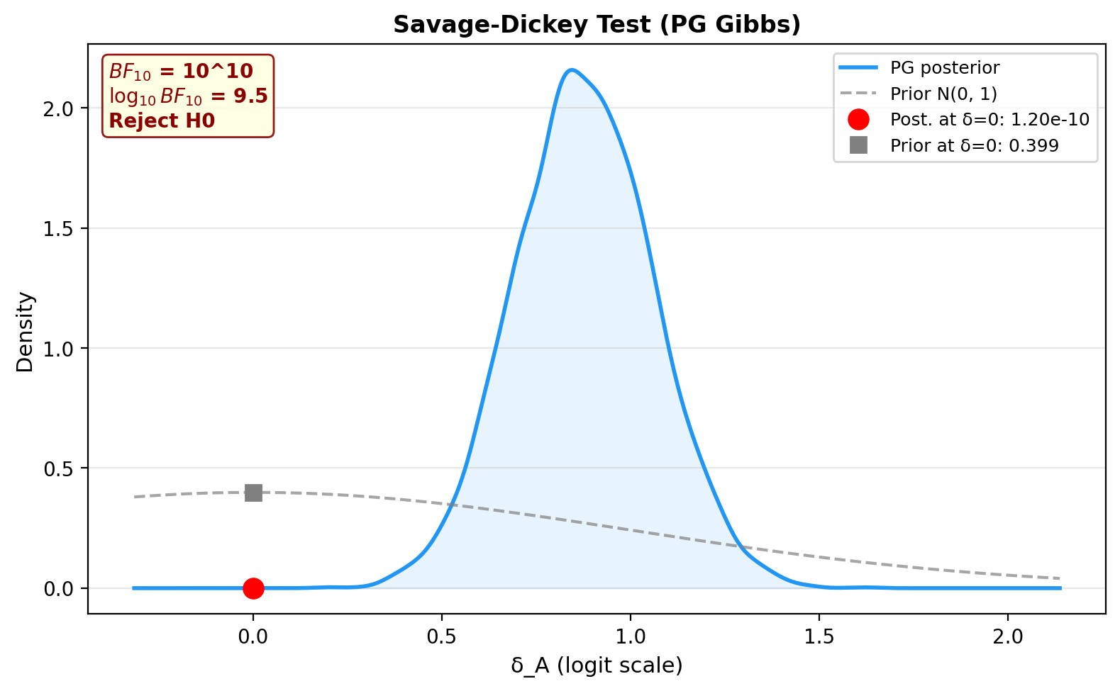
Bayes Factor:   BF₁₀ = 10^27   → Reject H0
Posterior Null: P(H₀|D) = 0.0000  → Reject H0
ROPE:           Reject H0 — A practically better  (0.0% in ROPE)
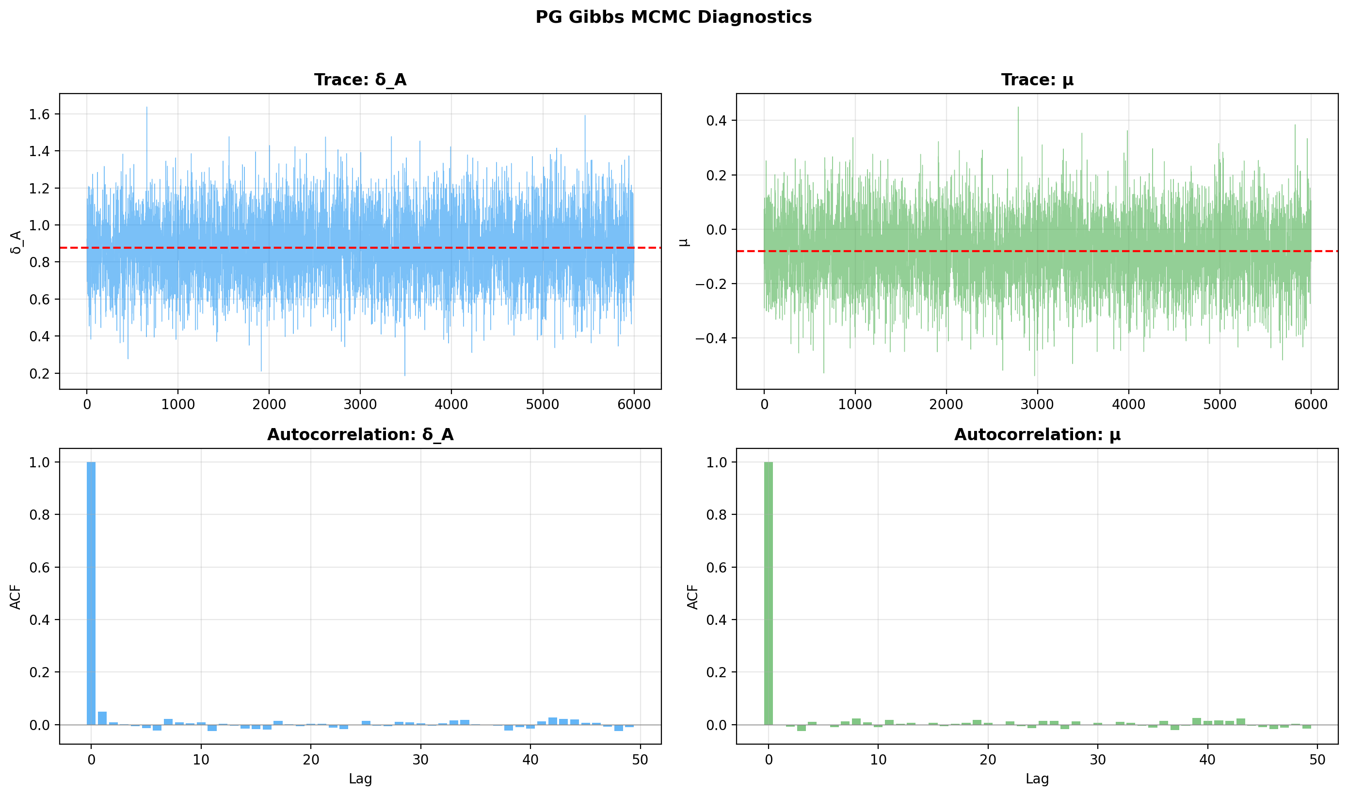
4. MCMC diagnostics
Two standard diagnostics summarise sampler health:
- R-hat (Gelman-Rubin) compares between- and within-chain variance; values close to 1 (target \(\hat{R} < 1.05\)) indicate the chains have mixed to the same distribution.
- ESS (effective sample size) is the number of independent draws equivalent to the autocorrelated MCMC sample; target ESS > 400 per parameter for stable posterior summaries.
Convergence checks
Always verify that R-hat < 1.05 and ESS > 400 before
trusting the results. If convergence is poor, increase n_iter
or n_chains.
diag = pg_model.mcmc_diagnostics()
print(f"μ:   R-hat={diag.mu.r_hat:.3f}, ESS={diag.mu.ess:.0f}")
print(f"δ_A: R-hat={diag.delta_A.r_hat:.3f}, ESS={diag.delta_A.ess:.0f}")
5. Trace and autocorrelation plots
Use the built-in trace plot — it renders all chains together, with per-parameter trace and ACF panels:
6. Savage-Dickey Bayes Factor
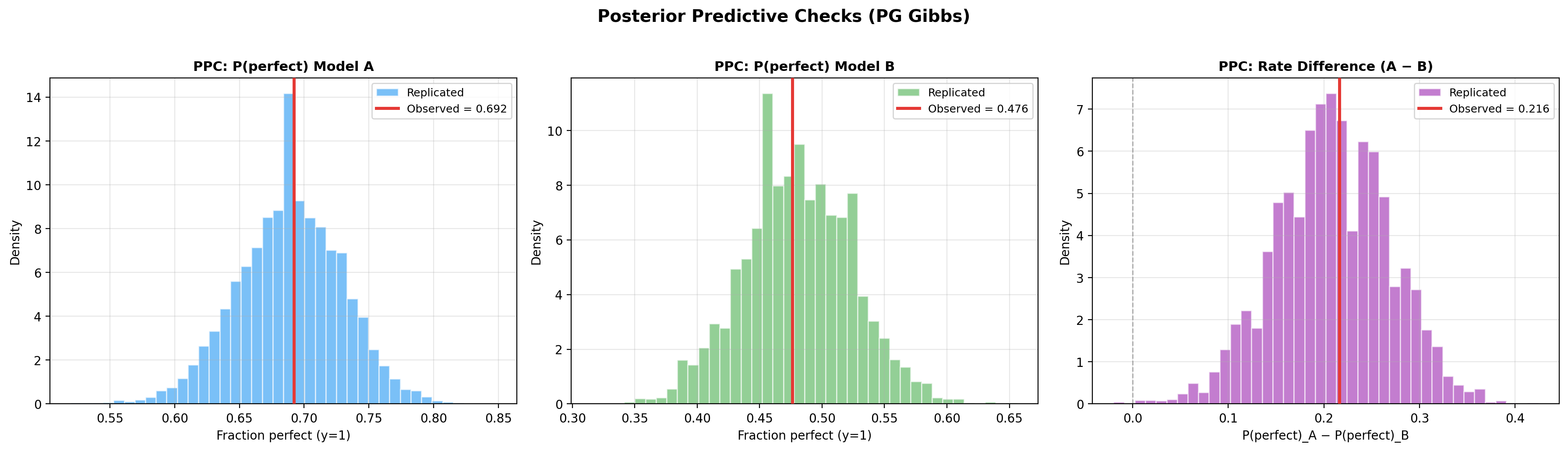
7. Posterior predictive checks
pg_model.plot_ppc(seed=42)

ppc = pg_model.ppc_pvalues(seed=42)
print(f"{'Statistic':<20} {'Observed':>10} {'p-value':>10} {'Status':>10}")
print("-" * 55)
for stat_name, vals in ppc.items():
    print(f"{stat_name:<20} {vals.observed:>10.4f} {vals.p_value:>10.3f} {vals.status:>10}")
Comparison with Laplace
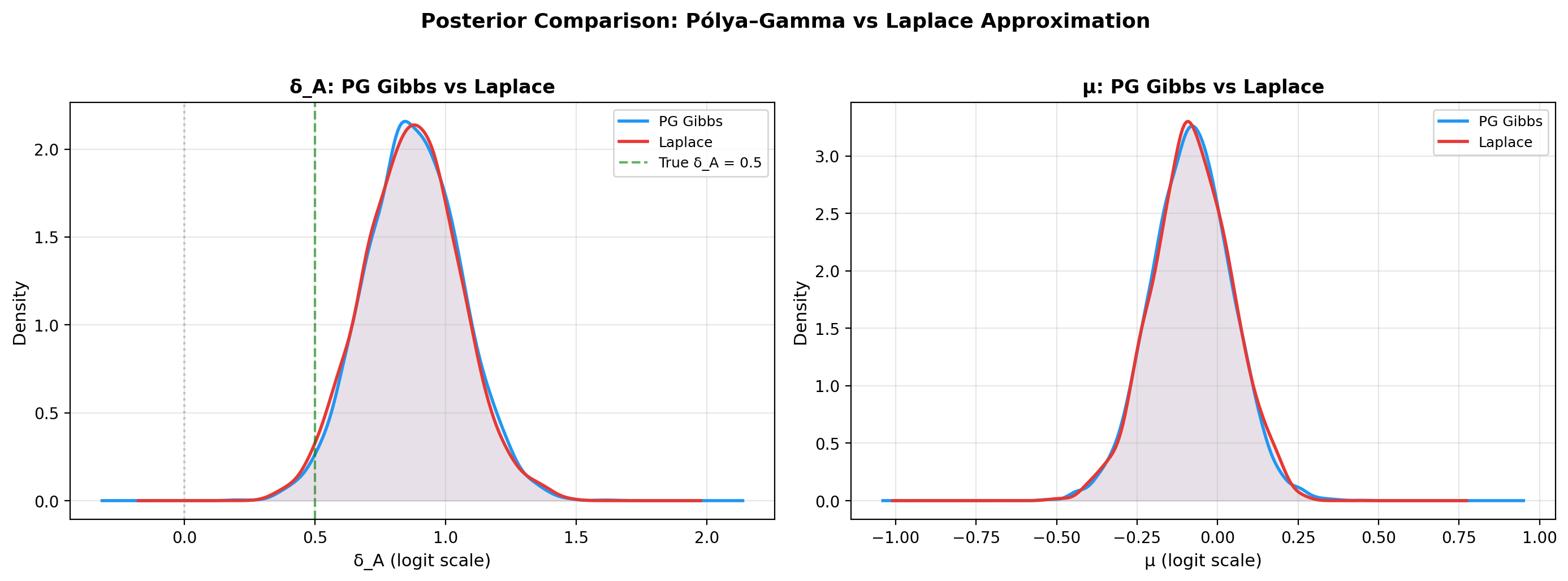
A key use case for the PG sampler is to verify that the Laplace approximation gives similar results. Fit both on the same data and compare:
laplace_model = PairedBayesPropTest(seed=42, n_samples=2000).fit(y_A, y_B)

delta_samples = pg_model.delta_A_samples
mu_samples = pg_model.samples[:, 0]
laplace_delta = laplace_model.delta_A_samples
laplace_mu = laplace_model.laplace["mu_samples"]

print("PG Gibbs vs Laplace — posterior summary")
print("=" * 55)
print(f"{'':20} {'PG Gibbs':>15} {'Laplace':>15}")
print("-" * 55)
print(f"{'δ_A mean':20} {delta_samples.mean():>15.4f} {laplace_delta.mean():>15.4f}")
print(f"{'δ_A sd':20} {delta_samples.std():>15.4f} {laplace_delta.std():>15.4f}")
print(f"{'μ mean':20} {mu_samples.mean():>15.4f} {laplace_mu.mean():>15.4f}")
print("=" * 55)
PG Gibbs vs Laplace: posterior KDEs of μ and δ_A
import matplotlib.pyplot as plt
from scipy.stats import gaussian_kde

fig, axes = plt.subplots(1, 2, figsize=(14, 5))

# δ_A comparison
ax = axes[0]
for samples, label, color in [
    (delta_samples, "PG Gibbs", "#2196F3"),
    (laplace_delta, "Laplace", "#E53935"),
]:
    kde = gaussian_kde(samples)
    x = np.linspace(samples.min() - 0.5, samples.max() + 0.5, 300)
    ax.plot(x, kde(x), linewidth=2, color=color, label=label)
    ax.fill_between(x, kde(x), alpha=0.1, color=color)

ax.axvline(1.0, color="green", ls="--", alpha=0.6, label="True δ_A = 1.0")
ax.axvline(0, color="gray", ls=":", alpha=0.4)
ax.set_xlabel("δ_A (logit scale)")
ax.set_title("δ_A: PG Gibbs vs Laplace", fontweight="bold")
ax.legend(fontsize=9)
ax.grid(alpha=0.3)

# μ comparison
ax = axes[1]
for samples, label, color in [
    (mu_samples, "PG Gibbs", "#2196F3"),
    (laplace_mu, "Laplace", "#E53935"),
]:
    kde = gaussian_kde(samples)
    x = np.linspace(samples.min() - 0.5, samples.max() + 0.5, 300)
    ax.plot(x, kde(x), linewidth=2, color=color, label=label)
    ax.fill_between(x, kde(x), alpha=0.1, color=color)

ax.set_xlabel("μ (logit scale)")
ax.set_title("μ: PG Gibbs vs Laplace", fontweight="bold")
ax.legend(fontsize=9)
ax.grid(alpha=0.3)

fig.suptitle("Posterior Comparison: Pólya–Gamma vs Laplace",
             fontsize=13, fontweight="bold", y=1.02)
plt.tight_layout()
plt.show()
Savage-Dickey comparison
d_pg = pg_model.decide()
d_lp = laplace_model.decide()

print(f"{'':20} {'PG Gibbs':>15} {'Laplace':>15}")
print("-" * 55)
print(f"{'BF₁₀':20} {d_pg.bayes_factor.BF_10:>15.2f} {d_lp.bayes_factor.BF_10:>15.2f}")
print(f"{'BF Decision':20} {d_pg.bayes_factor.decision:>15} {d_lp.bayes_factor.decision:>15}")
print(f"{'ROPE Decision':20} {d_pg.rope.decision:>15} {d_lp.rope.decision:>15}")
| Aspect | Laplace | Pólya-Gamma |
|---|---|---|
| Speed | Fast (milliseconds) | Slower (seconds) |
| Accuracy | Approximate | Exact (up to MCMC) |
| Diagnostics | None | R-hat, ESS |
| Recommended for | Exploration | Final reporting |
Unified decision comparison
print("Unified Decision — PG Gibbs vs Laplace")
print("=" * 70)

for label, m in [("PG Gibbs", pg_model), ("Laplace", laplace_model)]:
    d = m.decide()
    bf = d.bayes_factor
    pn = d.posterior_null
    rp = d.rope

    print(f"\n{label}:")
    print(f"  Bayes Factor:    BF₁₀ = {bf.BF_10:.2f}  → {bf.decision}")
    print(f"  Posterior Null:   P(H₀|D) = {pn.p_H0:.4f}  → {pn.decision}")
    print(f"  ROPE [{rp.rope_lower:.2f}, {rp.rope_upper:.2f}]:  "
          f"{rp.decision}  ({rp.pct_in_rope:.1%} in ROPE)")
BFDA sample-size planning
from bayesprop.utils.utils import (
bfda_power_curve,
plot_bfda_power,
plot_bfda_sensitivity,
)
theta_A_hat = y_A.mean()
theta_B_hat = y_B.mean()
sample_sizes = [20, 30, 50, 75, 100, 150, 200, 300, 500]
power_curve = bfda_power_curve(
theta_A_true=theta_A_hat,
theta_B_true=theta_B_hat,
sample_sizes=sample_sizes,
design="paired",
decision_rule="bayes_factor",
bf_threshold=3.0,
n_sim=200,
n_iter=1000,
burn_in=300,
n_chains=2,
seed=42,
)
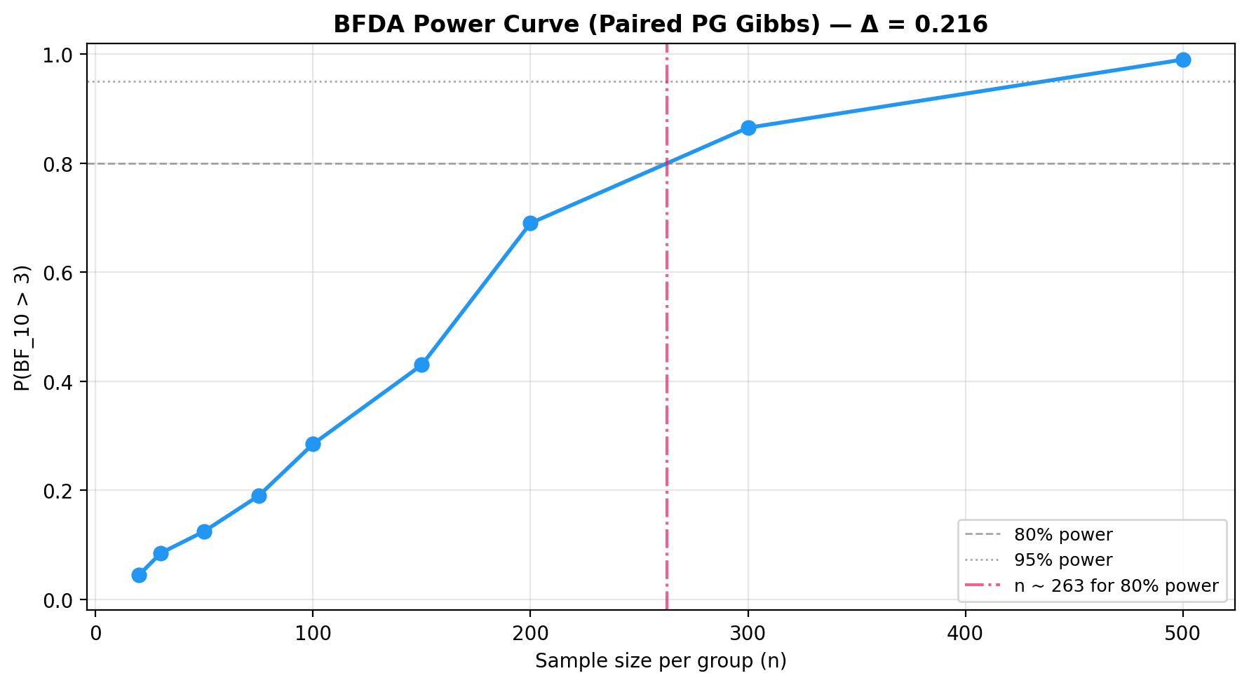
plot_bfda_power(
power_curve, theta_A_hat, theta_B_hat,
title=f"BFDA Power Curve (Paired PG Gibbs) — Δ = {theta_A_hat - theta_B_hat:.3f}"
)
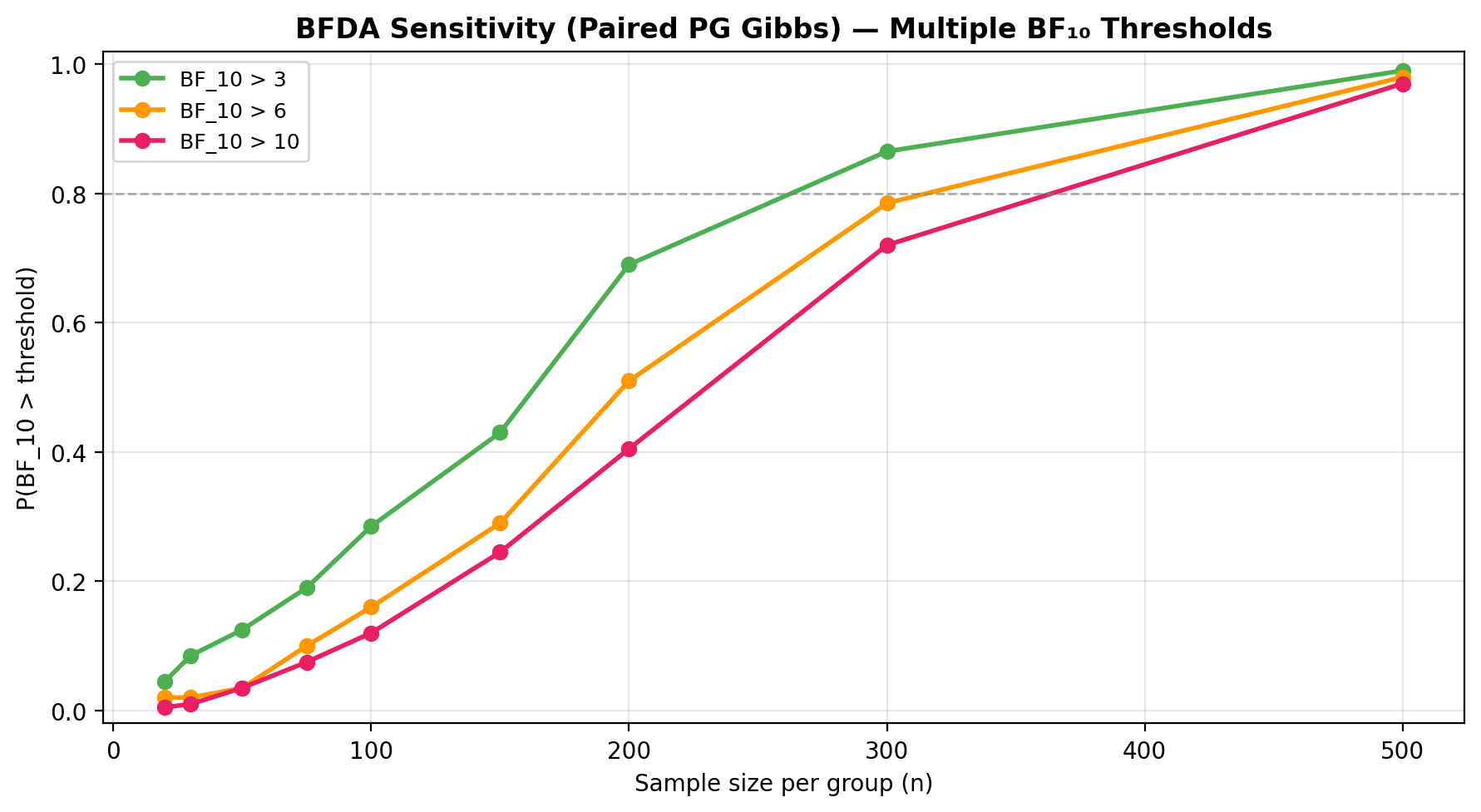
Sensitivity to BF threshold:
plot_bfda_sensitivity(
    theta_A_true=theta_A_hat,
    theta_B_true=theta_B_hat,
    sample_sizes=sample_sizes,
    thresholds=[3.0, 6.0, 10.0],
    n_sim=200,
    seed=42,
    design="paired",
    title="BFDA Sensitivity — Multiple BF₁₀ Thresholds",
)
See the BFDA guide for the full sample-size planning workflow.
Hierarchical example
The hierarchical variant uses the same unified facade — just
pass hyperprior_mu and hyperprior_delta (see the
hierarchical model and
extended Gibbs sampler above).
from bayesprop.resources.bayes_paired import PairedBayesPropTest
from bayesprop.resources.bayes_paired_laplace import _format_bf
from bayesprop.utils.utils import simulate_paired_scores
import numpy as np

sim = simulate_paired_scores(N=250, theta_A=0.69, theta_B=0.50, seed=42)

pg_hier = PairedBayesPropTest(
    method="pg",
    seed=42,
    n_iter=2000,
    burn_in=500,
    n_chains=4,
    hyperprior_mu=(2.0, 1.0),      # IG(2, 1) on σ²_μ
    hyperprior_delta=(2.0, 1.0),   # IG(2, 1) on σ²_δ
).fit(sim.y_A, sim.y_B)

pg_hier.print_summary()
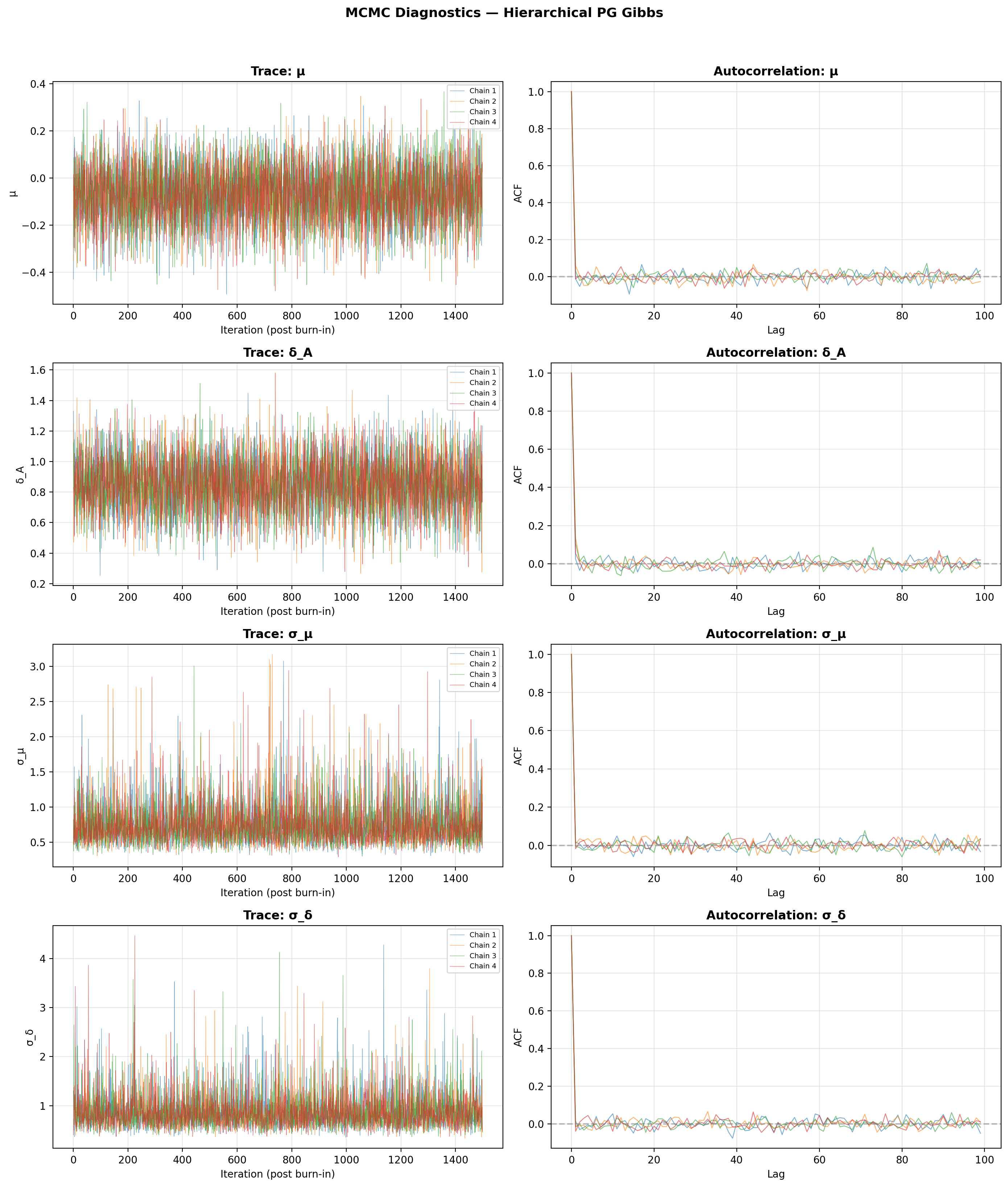
MCMC diagnostics (hierarchical)
The trace plot automatically adds rows for \(\sigma_\mu\) and \(\sigma_\delta\) when hyperpriors are active:
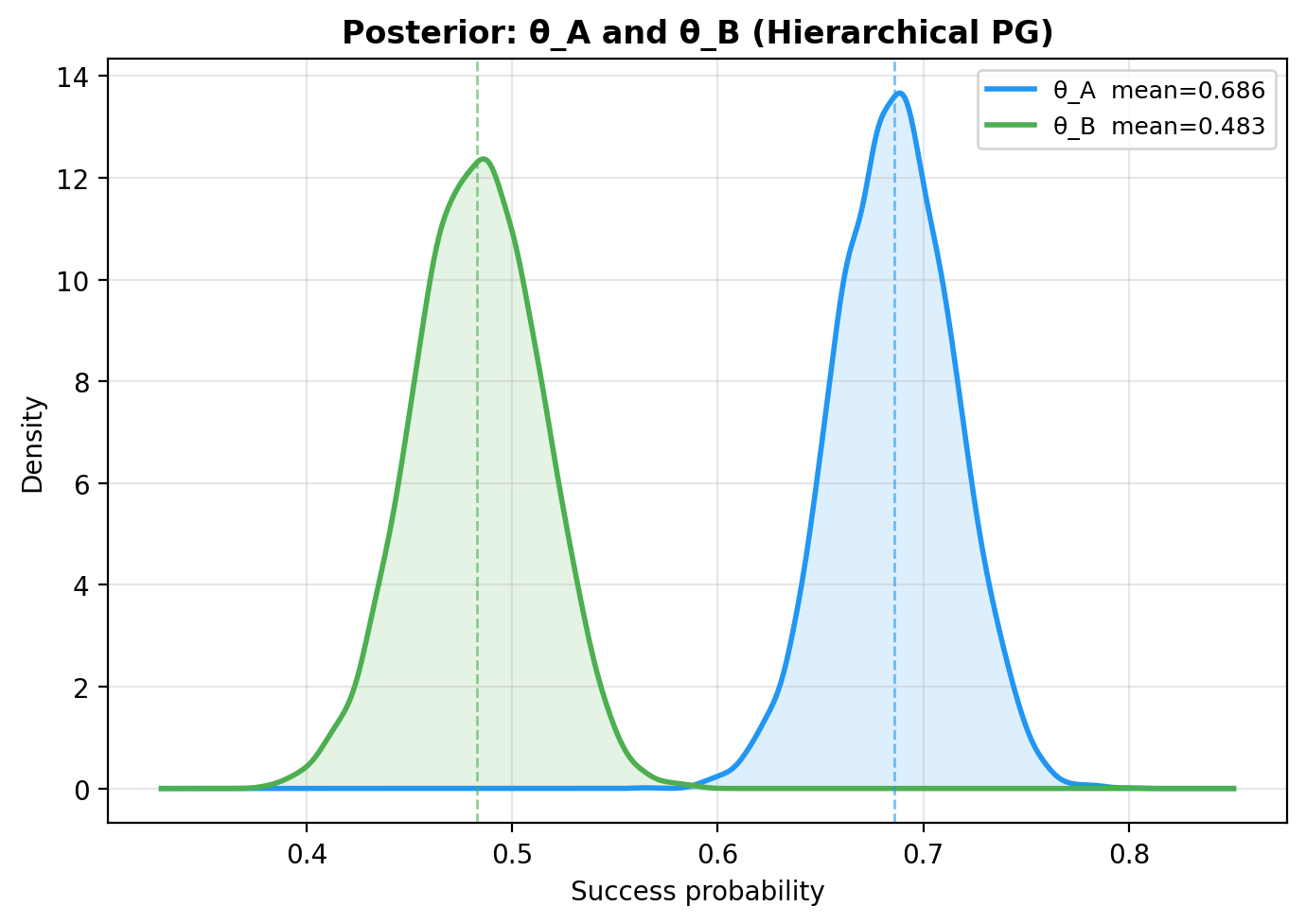
Posterior KDEs
Unified decision (hierarchical)
The Savage-Dickey Bayes factor automatically uses the marginal Student-\(t\) prior on \(\delta_A\) induced by the IG hyperprior:
d = pg_hier.decide()
bf = d.bayes_factor

print(f"BF₁₀ = {_format_bf(bf.BF_10)}  →  {bf.decision}")
print(f"log₁₀(BF₁₀) = {np.log10(bf.BF_10):.1f}")
print(f"Posterior Null: P(H₀|D) = {d.posterior_null.p_H0:.4f}  → {d.posterior_null.decision}")
print(f"ROPE: {d.rope.decision}  ({d.rope.pct_in_rope:.1%} in ROPE)")
Learned prior scales
The fitted model stores the posterior samples of \(\sigma_\mu^2\) and \(\sigma_\delta^2\):
sig_mu = np.sqrt(pg_hier.sigma_sq_mu_samples)
sig_delta = np.sqrt(pg_hier.sigma_sq_delta_samples)

print(f"Learned σ_μ:  mean = {sig_mu.mean():.3f}  "
      f"95% CI = [{np.quantile(sig_mu, 0.025):.3f}, {np.quantile(sig_mu, 0.975):.3f}]")
print(f"Learned σ_δ:  mean = {sig_delta.mean():.3f}  "
      f"95% CI = [{np.quantile(sig_delta, 0.025):.3f}, {np.quantile(sig_delta, 0.975):.3f}]")
Fixed vs Hierarchical comparison
# Fit a fixed-prior model for comparison
pg_fixed = PairedBayesPropTest(method="pg", seed=42).fit(sim.y_A, sim.y_B)

d_fix = pg_fixed.decide()
bf_fix = d_fix.bayes_factor

print(f"{'':25} {'Fixed':>18} {'Hierarchical':>18}")
print("-" * 65)
print(f"{'Mean Δ (θ_A − θ_B)':25} {pg_fixed.summary.mean_delta:>18.4f} {pg_hier.summary.mean_delta:>18.4f}")
print(f"{'P(A > B)':25} {pg_fixed.summary.p_A_greater_B:>18.4f} {pg_hier.summary.p_A_greater_B:>18.4f}")
print(f"{'log₁₀(BF₁₀)':25} {np.log10(bf_fix.BF_10):>18.1f} {np.log10(bf.BF_10):>18.1f}")
print(f"{'BF₁₀':25} {_format_bf(bf_fix.BF_10):>18} {_format_bf(bf.BF_10):>18}")
print(f"{'BF Decision':25} {bf_fix.decision:>18} {bf.decision:>18}")
When to use the hierarchical variant
- You are unsure about a sensible value for \(\sigma_\delta\) and want the data to inform it rather than commit to a fixed slab width.
- You want a Bayes factor that is robust to the prior-sensitivity / Jeffreys–Lindley paradox.
- You have enough data (\(n \gtrsim 50\)) for the IG posteriors to concentrate.
- You want full posterior uncertainty on the prior scales (MCMC gives you the entire posterior distribution, not just a MAP point estimate as in the Laplace variant).
For a fixed-prior analysis where you deliberately choose \(\sigma_\delta\),
set hyperprior_mu=None, hyperprior_delta=None (the default).
Inputs and binarisation
PairedBayesPropTest(method="pg") accepts both already-binary {0, 1} inputs and
continuous scores in [0, 1]. Continuous inputs are auto-binarised at a
configurable threshold (default 0.5):
Values strictly outside [0, 1] or NaN raise ValueError instead of
being silently truncated. Pass already-binarised arrays for the fast path.
API
See API Reference — Paired Model (Pólya-Gamma) for full method documentation.
References
- Polson, N. G., Scott, J. G. & Windle, J. (2013). Bayesian inference for logistic models using Pólya-Gamma latent variables. Journal of the American Statistical Association, 108(504), 1339–1349.
- Windle, J., Polson, N. G. & Scott, J. G. (2014). Sampling Pólya-Gamma random variates: alternate and approximate techniques. arXiv:1405.0506.