Titanic data set example

Note: The focus of this example is less on finding anomalies but rather to illustrate model explanability in the case of categorical and continuous features.

import numpy as np
from sklearn.datasets import fetch_openml
from bhad.model import BHAD

X, y = fetch_openml("titanic", version=1, as_frame=True, return_X_y=True)

X.head(2)

	pclass	name	sex	age	sibsp	parch	ticket	fare	cabin	embarked	boat	body	home.dest
0	1	Allen, Miss. Elisabeth Walton	female	29.0000	0	0	24160	211.3375	B5	S	2	NaN	St Louis, MO
1	1	Allison, Master. Hudson Trevor	male	0.9167	1	2	113781	151.5500	C22 C26	S	11	NaN	Montreal, PQ / Chesterville, ON

X_cleaned = X.drop(['body', 'cabin', 'name', 'ticket', 'boat'], axis=1).dropna()  # not needed
y_cleaned = y[X_cleaned.index]

X_cleaned.info(verbose=True)

<class 'pandas.core.frame.DataFrame'>
Index: 684 entries, 0 to 1281
Data columns (total 8 columns):
 #   Column     Non-Null Count  Dtype
---  ------     --------------  -----
 0   pclass     684 non-null    int64
 1   sex        684 non-null    category
 2   age        684 non-null    float64
 3   sibsp      684 non-null    int64
 4   parch      684 non-null    int64
 5   fare       684 non-null    float64
 6   embarked   684 non-null    category
 7   home.dest  684 non-null    object
dtypes: category(2), float64(2), int64(3), object(1)
memory usage: 39.0+ KB

Partition dataset:

from sklearn.model_selection import train_test_split

X_train, X_test, y_train, y_test = train_test_split(X_cleaned, y_cleaned, test_size=0.33, random_state=42)

print(X_train.shape)
print(X_test.shape)

print(np.unique(y_train, return_counts=True))
print(np.unique(y_test, return_counts=True))

(458, 8)
(226, 8)
(array(['0', '1'], dtype=object), array([242, 216]))
(array(['0', '1'], dtype=object), array([122, 104]))

Train model and create local/global model explanation:

Retrieve local model explanations. Here: Specify all numeric and categorical columns explicitly

num_cols = list(X_train.select_dtypes(include=['float', 'int']).columns)
cat_cols = list(X_train.select_dtypes(include=['object', 'category']).columns)

Score your train set:

model = BHAD(
    contamination=0.01,
    num_features=num_cols,
    cat_features=cat_cols,
    nbins=None,
    verbose=False
)

y_pred_train_new = model.fit_predict(X_train)
scores_train_new = model.decision_function(X_train)

print("Training predictions:", np.unique(y_pred_train_new, return_counts=True))

Training predictions: (array([-1,  1]), array([  5, 453]))

from bhad import explainer

local_expl = explainer.Explainer(bhad_obj=model, discretize_obj=model._discretizer).fit()

--- BHAD Model Explainer ---

Using fitted BHAD and discretizer.
Marginal distributions estimated using train set of shape (458, 8)

df_train = local_expl.get_explanation(nof_feat_expl = 5)

Create local explanations for 458 observations.

global_feat_imp = local_expl.global_feat_imp         # based on X_train
global_feat_imp

	avg ranks
embarked	0.152058
sex	0.257304
parch	0.279548
sibsp	0.444223
age	0.491700
fare	0.546813
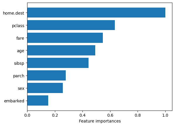
pclass	0.634462
home.dest	1.000000

Get global model explanation (in decreasing order):

from matplotlib import pyplot as plt

plt.barh(global_feat_imp.index, global_feat_imp.values.flatten())
plt.xlabel("Feature importances");

Get local explanations, i.e. feature importances (in decreasing order):

for obs, ex in enumerate(df_train.explanation.values):
    if (obs % 100) == 0:
        print(f'\nObs. {obs}:\n', ex)

Obs. 0:
 parch (Cumul.perc.: 0.996): 5.0
home.dest (Perc.: 0.011): Sweden Winnipeg, MN
sex (Perc.: 0.4): female

Obs. 100:
 home.dest (Perc.: 0.002): Tofta, Sweden Joliet, IL
fare (Cumul.perc.: 0.07): 7.78

Obs. 200:
 home.dest (Perc.: 0.013): Brooklyn, NY

Obs. 300:
 home.dest (Perc.: 0.007): Bournmouth, England
age (Cumul.perc.: 0.05): 5.0
sex (Perc.: 0.4): female

Obs. 400:
 home.dest (Perc.: 0.002): Taalintehdas, Finland Hoboken, NJ

y_pred_test = model.predict(X_test)

df_test = local_expl.get_explanation(nof_feat_expl = 4)
df_test.head(2)

Create local explanations for 226 observations.

	pclass	sex	age	sibsp	parch	fare	embarked	home.dest	explanation
0	2.0	male	36.0	1.0	2.0	27.7500	S	Bournmouth, England	home.dest (Perc.: 0.007): Bournmouth, England
1	1.0	male	49.0	1.0	1.0	110.8833	C	Haverford, PA	home.dest (Perc.: 0.007): Haverford, PA\nfare ...

for obs, ex in enumerate(df_test.explanation.values):
    if (obs % 50) == 0:
        print(f'\nObs. {obs}:\n', ex)

Obs. 0:
 home.dest (Perc.: 0.007): Bournmouth, England

Obs. 50:
 home.dest (Perc.: 0.002): Deephaven, MN / Cedar Rapids, IA
fare (Cumul.perc.: 0.91): 106.42

Obs. 100:
 home.dest (Perc.: 0.002): Hudson, NY
sex (Perc.: 0.4): female

Obs. 150:
 home.dest (Perc.: 0.0): ?Havana, Cuba

Obs. 200:
 embarked (Perc.: 0.048): Q
home.dest (Perc.: 0.0): Co Sligo, Ireland Hartford, CT
sex (Perc.: 0.4): female
fare (Cumul.perc.: 0.061): 7.75

local_expl.global_feat_imp   # based on X_test

	avg ranks
embarked	0.157711
parch	0.245639
sex	0.256804
sibsp	0.441731
age	0.480112
fare	0.575715
pclass	0.638521
home.dest	1.000000